
Grantee Research Project Results
2011 Progress Report: Integrating Future Climate Change and Riparian Land-Use to Forecast the Effects of Stream Warming on Species Invasions and Their Impacts on Native Salmonids
EPA Grant Number: R833834Title: Integrating Future Climate Change and Riparian Land-Use to Forecast the Effects of Stream Warming on Species Invasions and Their Impacts on Native Salmonids
Investigators: Olden, Julian D. , Lawler, Joshua J. , Torgersen, Christian E.
Current Investigators: Olden, Julian D. , Torgersen, Christian E. , Lawler, Joshua J.
Institution: University of Washington , USGS Forest and Rangeland Ecosystem Science Center
Current Institution: University of Washington , Northwest Fisheries Science Center
EPA Project Officer: Packard, Benjamin H
Project Period: July 1, 2008 through June 30, 2012 (Extended to June 30, 2013)
Project Period Covered by this Report: July 1, 2010 through June 30,2011
Project Amount: $587,209
RFA: Ecological Impacts from the Interactions of Climate Change, Land Use Change and Invasive Species: A Joint Research Solicitation - EPA, USDA (2007) RFA Text | Recipients Lists
Research Category: Climate Change , Aquatic Ecosystems
Objective:
Climate change, increasing agricultural and urban land-use, and invasive species threaten the functioning of freshwater ecosystems in the Pacific Northwest of the United States. Resource managers, scientists and policy makers are becoming increasingly cognizant that the future will witness simultaneous changes in these factors, yet we still lack the science and decision-support tools required to develop management strategies that are robust to future environmental change. Our project seeks to develop an analytical framework for linking climate change, riparian land-use, stream thermodynamics, and species invasions for the management and conservation of freshwater ecosystems. We demonstrate this framework for the John Day River, Oregon, where human-induced stream warming is promoting the range expansion of invasive smallmouth bass (Micropterus dolomieu) and northern pikeminnow (Ptychocheilus oregonensis) into formerly uninhabitable reaches that contain critical migration, spawning, and rearing habitat for endangered Chinook salmon (Oncorhynchus tshawytscha). Our proposal has three objectives. First, we will characterize and develop predictive models that forecast spatiotemporal patterns of riverine thermal regimes in response to future climate change and riparian land-use. Second, we will forecast species-specific responses (range contractions and invasions) to projected future thermal regimes. Third, we will evaluate alternative scenarios of climate change to identify critical areas for riparian habitat restoration and protection to mediate future climate-induced warming of streams and species invasions.
Progress Summary:
Research Element 1: Develop climate-change projections
This task has been completed and was summarized in the 2009 Annual Report.
Research Element 2: Characterize riparian land cover and geomorphology
This task has been completed and was summarized in the 2010 Annual Report.
Research Element 3: Quantify multi-scaled thermal regimes
This task has been completed and was summarized in the 2010 Annual Report.
Research Element 4: Develop a spatially explicit stream temperature model
We have built a geostatistical network model of stream temperature to forecast potential climate-induced changes in the availability of thermally suitable habitat for our focal species. Details are provided below.
Stream temperature modeling
At each site, for each summer, we calculated the maximum weekly mean stream temperature (MWMST) as:
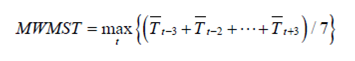
where T is the mean temperature observation at day t. Stream temperature data were primarily compiled by the Northwest Fisheries Science Center (National Oceanic Atmospheric Administration) (246 independent data collection events from 1993 to 2007). To augment this dataset, we collected stream temperature data using digital temperature loggers (Onset data logger models: Tidbit, Water Temp Pro, and Hobo Pendant) during the summer of 2009 (52 independent data collection events). All data collection events represented continuous sampling from June 21 through September 21, with a sampling interval ≤ 60 minutes, and MWMST ≤ 30°C (Dunham et al. 2005).
We compiled a set of candidate predictors of stream temperature previously identified in the literature (Caissie 2006; Webb et al. 2008) and attributed them to the NHDPlus geospatial dataset (Environmental Protection Agency & Horizon Systems Corporation 2008). Most predictor variables were retrieved from NHDPlus value-added attribute tables. Variables not included in the NHDPlus geospatial dataset were computed using a combination of ArcGIS Desktop version 9.3.1 (Environmental Systems Research Institute 1999), NHDPlus CA3T (Horizon Systems Corporation 2008), and R statistical software (R Development Core Team 2010). We identified covariates of MWMST by visually analyzing bivariate scatterplots, log-transforming predictor variables with skewed distributions, and excluding those with a Pearson’s correlation coefficient of less than 0.1.
Variables that fit the above criteria (i.e., cumulative riparian solar exposure and maximum weekly mean air temperature) are described below. Cumulative riparian solar exposure (CSRE) was derived from three datasets: mean annual solar radiation (modeled using ArcGIS Solar Analyst), LANDFIRE percent canopy cover (Rollins et al. 2006), and potential riparian land-cover extracted from the LANDFIRE biophysical settings dataset. LANDFIRE potential riparian land-cover types were derived using a supervised predictive modeling approach that links existing vegetation with gradients of climate, topography, and soils (Rollins et al. 2006). CRSE was computed using the equation:
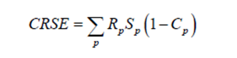
where riparian land-cover is represented by R (1 = riparian, 0 = non-riparian), solar radiation is represented by S, and percent canopy cover is represented by C, at every pth pixel. The product of RpSp(1-Cp) was then summed downstream using CA3T. To calculate maximum weekly maximum air temperature (MWMAT), we gathered daily observations from four Western Regional Climate Center Remote Automatic Weather Stations (WRCC RAWS, http://www.raws.dri.edu/): Case, Board Creek, Fall Mountain, and North Pole Ridge. For each year, Y, we calculated MWMAT as:
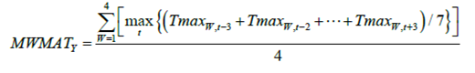
where t represents each day within that year, and W = 1,…,4 represents each of the four weather stations where temperature was observed.
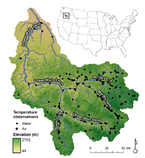
Figure 1. Map of the John Day River showing the spatial extent of the fish surveys of the North Fork and Middle fork.
Geostatistical network model of MWMST
Recent studies suggest that multiple patterns of spatial autocorrelation may be present in stream temperature data (Peterson et al. 2006; Isaak et al. 2010) and it was likely that our data would also be spatially autocorrelated given the relatively large number of observations collected within a single catchment. Analyzing spatially correlated data requires the use of spatial statistical methodologies because the assumption of independence is violated, making many conventional statistical methods inappropriate (Legendre 1993). Therefore, we built the stream temperature model using a new geostatistical modeling approach designed to represent the unique spatial configuration, longitudinal connectivity, flow volume and flow direction found in stream networks (Peterson & Ver Hoef 2010; Ver Hoef & Peterson 2010). This approach permits valid autocovariances to be generated based on a variety of hydrologic, or watercourse (Olden et al. 2001; Ganio et al. 2005), relationships. “Tail-up” covariances are based on watercourse distance, but restrict correlation to “flow-connected” locations (e.g., water flows from an upstream location to a downstream location). Spatial weights are also incorporated into the tail-up model to account for the disproportionate influence that large tributaries may have on downstream locations. “Tail-down” covariances restrict correlation to locations that reside on the same stream network (e.g., two locations share a common outlet), with correlation permitted between both flow-connected and flow-unconnected locations (e.g., two locations are on the same network, but are not flow-connected). In addition, a mixed-modeling approach can be used in conjunction with these methods, which provides a way to model spatially correlated errors using both Euclidean and watercourse distance measures in a single model (Ver Hoef & Peterson 2010).
The model selection process was implemented in two steps: first, non-spatial linear models were used to select a subset of predictor variables for inclusion in the geostatistical model; second, spatial autocovariance models were selected based on prediction performance. Multivariate, additive, first-order, non-spatial linear models were fit using a forward stepwise regression approach (Neter et al. 1983) and compared using Akaike’s Information Criterion (AIC, Sakamoto et al. 1986). The variables contained in the model with the lowest AIC value were then used as the predictors in the geostatistical models. Once the most suitable subset of predictor variables had been identified, a suite of geostatistical models were fit and compared to find the combination of autocovariance models that produced the best model predictions. The pair-wise watercourse distances and spatial weights needed to fit a geostatistical model were generated using the Functional Linkage of Waterbasins and Streams (FLoWS) ArcGIS toolset (Theobald et al. 2006), as well as custom scripts written in Python version 2.4.1 (Van Rossum 2008). The spatial weights were based on contributing area (Peterson & Ver Hoef 2010; Isaak et al. 2010), which we used as a proxy for flow (i.e., discharge). In total, seven geostatistical models were fit using R statistical software (R Development Core Team 2006), representing every linear combination of the three autocovariance functions (Euclidean Spherical, Linear-with-sill tail-down and Exponential tail-up). The geostatistical models were mixed-models, meaning that they included the exponential tail-down and spherical Euclidean autocovariance functions (Ver Hoef & Peterson 2010). Each model contained the same set of predictor variables, which were selected in Step 1. Leave-one-out cross-validation predictions were generated for each model and used to calculate the root mean square prediction error (RMSPE), as well as the squared Pearson correlation (r2) between the observations and the predictions. The model with the lowest RMSPE was then selected as the “final” model.
Results
The most likely network model included cumulative riparian solar exposure (CRSE) and maximum weekly maximum air temperature (MWMAT), both of which were positively related to MWMST (Table 1). Both explanatory variables were highly significant (p < 0.001), but of the two, CRSE explained a greater percent of total variation. The geostatistical model was considerably more accurate than the non-spatial linear regression with the same predictor variables (R2=0.84 vs. R2=0.69). The model that produced the most accurate predictions, based on the RMSPE, included the exponential tail-down and the spherical Euclidean models (the tail-up model did not lower RMSPE). The tail-down spatial component explained the majority of spatial variation (Table 1).
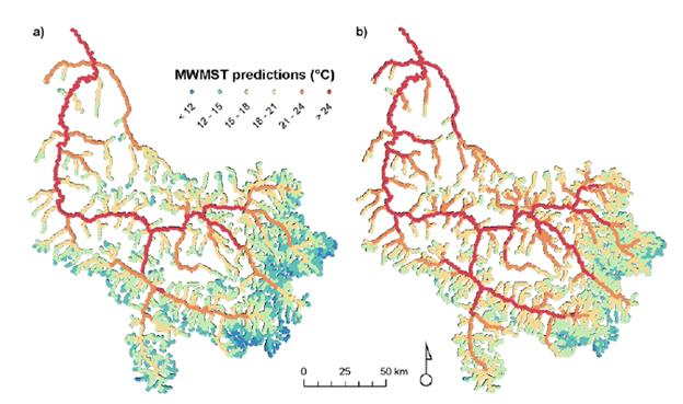
Modeled MWMST was coolest (10.4°C modeled, 9.2°C observed) in high elevation tributaries of the John Day River, and warmest (27.7°C modeled, 28.5°C observed) in the lower reaches of the North and Middle forks and throughout the lower main-stem (Fig. 2a). Between warm and cool summers, MWMST shifted as much as 2.4°C for the period 1993–2009 at any given location (corresponding to a shift of 3.8°C MWMAT). The warmest class of modeled stream temperature (>24°C MWMST, Fig. 2a) denotes stream reaches that are above the thermal tolerance for rainbow trout and Chinook salmon for an average year between 1993 and 2009.
| Variance componentb | ||||||||||||
|---|---|---|---|---|---|---|---|---|---|---|---|---|
| Parameters | n | Units | Min. | Max. | Mean | ß(SE) | t | r2 | RMPSEa | Fixed Effect | Spacial error (%) | |
| Intercept | -15.7(3.5) | -4.5 | 0.84 | 1.4 | 81.6 | tail-down | 13.7 | |||||
| log(CRSE) | 165 | log(Gigawatts/yr) | 1.8 | 13.9 | 9.2 | 1.4 (0.08) | 16.9 | Euclidean | 13.9 | |||
| MWMAT | 13 | 0C | 31.5 | 35.5 | 33.7 | 0.62 (0.09) | 6.7 | Nuggetc | 0.8 | |||
| total | 18.4 | |||||||||||
a Root mean square prediction error
b Variance component represents teh percent of variance explained by the parameters (fixed effect) and the autocovariance models used in
the geostatistical model (spacial error, Peterson & Ver Hoef 2010)
c Nugget represents error between observations pairs at zero distance from each other (i.e., sampling error or purely temporal error). Nugget
represents error between observations pairs a4t zero distance rom each other (i.e., smapling error or purely temporal error)
Research Element 5: Forecast future stream thermal regimes under scenarios of climate change
Methods
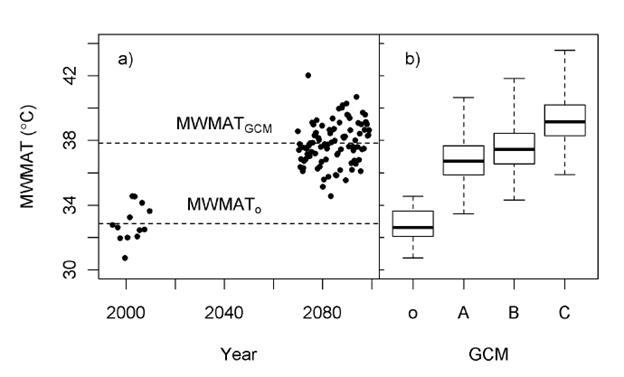
We used the final model and projected future air temperature (MWMAT) to generate three sets of future MWMST predictions. The future air temperatures were estimated using three different GCMs for a mid-range (A1B, Special Report on Emissions Scenarios, Solomon & IPCC 2007) greenhouse-gas emissions scenario. We chose the following GCMs based on their performance in the Pacific Northwest (Hamlet et al. 2010): ECHAM5/MPI-O, CNRM-CM3, and UKMO-HadCM3. We also wanted to compare future MWMST with present conditions; as such, we calculated a baseline MWMAT over the full observation period, MWMATo (average of all MWMAT observations between 1993 and 2009), and used those estimates to predict MWMST under typical MWMAT conditions (Fig. 3). We calculated future MWMAT (MWMATGCM) using spatially downscaled daily time-step climate projections (Mote & Salathe 2010). These data were downscaled from GCM cell resolution of typically 1–3° resolution (roughly 100-300 km at ±45° latitude) to a 1/16th degree resolution (6 km at ±45° latitude), and temporally downscaled from one month to daily temporal resolution using a “Hybrid Delta Approach” (Hamlet et al. 2010). At each of the four 1/16th degree cells that were positioned closest to the four weather stations in the John Day Basin (Fig. 1), we calculated a mean value of MWMAT across all years within the range of future variability. We then averaged the four mean values together to describe the MWMAT in the whole basin for an average year expected in the period 2070–2099.
Figure 2. Stream temperature predictions for average (a) historic (1993-2009) and (b) future (2070-2099) climate. Colors from red to blue represent modeled MWMST (final spatial model, see Table 1) for an average year (prediction based on average MWMAT across all observation years). Future predictions are based on an ensemble of the three GCMs that performed well for the Pacific Northwest. Prediction sites were placed in a network lattice with each site spaced at 2-km intervals.
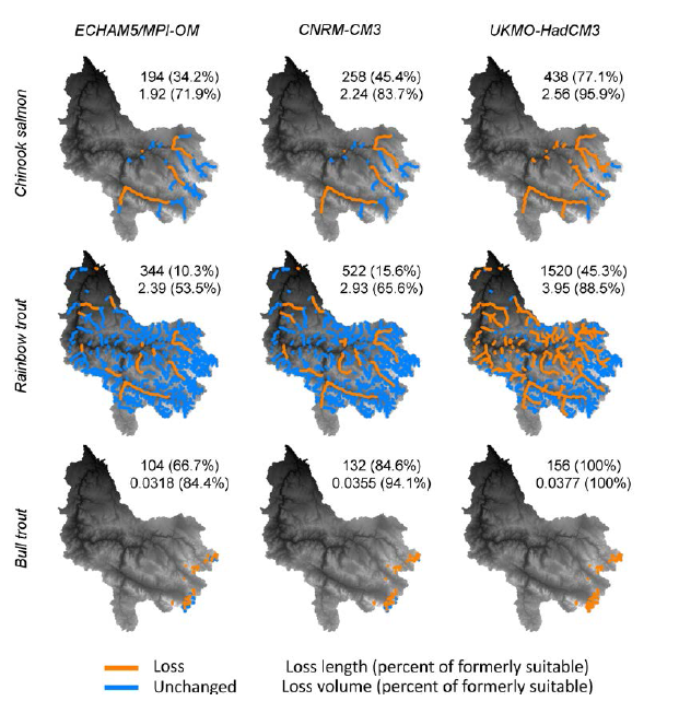
For each of the three values of MWMATGCM that corresponded to the three GCM estimates for the period 2070–99, we calculated the loss of habitat for each of the three species based on estimated thermal tolerances. We used a thermal tolerance of 24.0°C MWMST for Chinook salmon and rainbow trout (Eaton et al. 1995), where 24.0°C is the 95th percentile for a normal probability density function that corresponds to the mean, standard deviation, and sample size of MWMST for the sample set of observations for the species. We estimated a thermal tolerance of 14.4°C for bull trout using the same methods in Eaton et al. (1995) using a sample set of 237 bull trout observations corresponding to values of MWMST that were collected across the Columbia River Basin (Rieman & Chandler 1999). To ensure that we did not overestimate thermal habitat loss, we subtracted the length of intermittent stream (Environmental Protection Agency & Horizon Systems Corporation 2008; Oregon Department of Forestry 2011) and unoccupied habitat (based on sampling and best professional opinion, Oregon Department of Fish and Wildlife 2010) that overlapped with the predicted habitat that was lost due to climate change. We reported these estimates as both length and volume of stream habitat; volume was calculated by first multiplying length of habitat by modeled annual average flow (Jobson 1996) and then dividing by modeled annual average velocity (Jobson 1996).
Figure 3. A comparison of historical and projected future variability of maximum weekly mean air temperature (MWMAT): (a) scatterplots of historical (MWMATo) and future (MWMATGCM) MWMAT; (b) median, minimum, maximum, and inner quartile range of historical (o) and future (A, B, and C) MWMAT. The labels A, B, and C correspond to the following GCMs: A = ECHAM5/MPI-O, B = CNRM-CM3, and C = UKMO-HadCM3. MWMATGCM appears to vary more frequently than annually because the hybrid delta method (Hamlet et al. 2010) extracts the historical pattern of variability from the period 1915–2006 (i.e., 91 years of variability over the period 2070–2099).
Results
Projected MWMAT was predicted to increase by 5.0°C (based on a three-GCM ensemble average) by the period 2070–99. The geostatistical network model predicted that this change in air temperature would result in a change in stream temperature of 3.1°C MWMST (Fig. 2). The main-stem reaches of the John Day River show the most vulnerability to the loss of thermally suitable habitat because they have gradual thermal gradients (i.e., small changes in stream temperature can cause dramatic losses of thermally suitable habitat as shown by the shift of the warmest MWMST class along the main stem and North and Middle forks in Fig. 2). By comparison, headwater reaches were projected to experience less loss (i.e., MWMST analogues were closer in headwater streams).
Research Element 6: Model species responses of Chinook salmon, smallmouth bass and northern pikeminnow to future thermal regimes.
Our most recent product includes a map of potential habitat loss under the ECHAM5 SRES A2 climate change scenario for Chinook salmon, rainbow trout and bull trout (Figure 4). Similar models for bass and pikeminnow will be constructed using the temperature predictions from WET-Temp or HeatSource. We quantified potential habitat loss by comparing spatially continuous stream temperature maps for current and year 2080 stream temperature scenario. With this information, we located thermally marginal habitat for current normal conditions, and projected potential loss due to climate change for the year 2080. Our results indicate a significant potential compression of rearing habitat—40% of summer rearing habitat will be lost by the year 2080. Bridge Creek and Rock Creek, tributaries of the lower main stem that are currently marginally suitable, will lose all rearing habitat. Other warmer, drier streams, such as Mountain, Wall, and Cottonwood Creeks, will lose 70%, 80%, and 84% respectively. The least habitat will be lost in the upper North and Middle Forks. However, the upper North and Middle Forks are currently where the density of rearing salmonids is greatest. Therefore, even small losses of habitat will affect many individuals.
Figure 4. Projected loss of thermally suitable habitat by the period 2070-2099 under the A1B emissions scenario by GCM (ECHAM5/MPI-O, CNRM-CM3, and UKMO-HadCM3) and species (bull trout, rainbow trout, and Chinook salmon). Length of habitat lost is reported in kilometers and volume of habitat loss is reported in millions of cubic meters.
Research Element 7: Quantity the distribution of Chinook salmon, smallmouth bass and northern pikeminnow in response to longitudinal heterogeneity in thermal regimes
This task has been completed and was summarized in the 2010 Annual Report.
Other research activities
We have initiated a new project to investigate the behavioral and growth responses of juvenile Chinook salmon to smallmouth bass and northern pikeminnow using a series of mesocosm experiments conducted in an artificial stream channel. This research will provide insight into the mechanisms underpinning the patterns observed in the field, and thus is central to the outputs and outcomes from the EPA project. The first component of the project addresses the question: Are there differences in behavior and vulnerability of juvenile Chinook salmon to native, nonnative, and combined predators? This investigation takes a purely behavioral approach, and examines connections between the genetic basis of predator recognition, prey survival, and behavioral selection by predators. The second component is investigating the implications of increased temperature on the vulnerability of juvenile salmon to the direct (mortality) and indirect (reduced growth) effects of predation. Although many studies have been conducted on the separate effects of predation and temperature, the interaction of the two in a semi-natural environment has seldom been investigated. This integrated approach will fill a significant gap in knowledge of how predator-prey relationships will respond to climate change. Lastly, this study will be the first to compare anti-predator defenses of juvenile Chinook salmon to smallmouth bass (a species native to eastern North America and now present throughout Washington) and northern pikeminnow (a species native to select drainages in north-western North America but now expanding into new regions in the Columbia River Basin). In summary, we view this experimental work as a key data need to support the proposed objectives of the EPA project.
Journal Articles on this Report : 2 Displayed | Download in RIS Format
| Other project views: | All 38 publications | 28 publications in selected types | All 28 journal articles |
|---|
| Type | Citation | ||
|---|---|---|---|
|
|
Kuehne LM, Olden JD, Duda JJ. Costs of living for juvenile Chinook salmon (Oncorhynchus tshawytscha) in an increasingly warming and invaded world. Canadian Journal of Fisheries and Aquatic Sciences 2012;69(10):1621-1630. |
R833834 (2011) R833834 (2012) R833834 (Final) |
Exit Exit |
|
|
Ruesch AS, Torgersen CE, Lawler JJ, Olden JD, Peterson EE, Volk CJ, Lawrence DJ. Projected climate-induced habitat loss for salmonids in the John Day River Network, Oregon, U.S.A. Conservation Biology 2012;26(5):873-882. |
R833834 (2011) R833834 (2012) R833834 (Final) |
Exit Exit |
Supplemental Keywords:
Ecosystem protection/environmental exposure and risk, air, scientific discipline, climate change,ecological risk assessment, air pollution effects, atmosphere, aquatic ecosystem, monitoring/modeling, environmental monitoring, meteorology, climate model, global climate change, socioeconomics, ecosystem indicators, air quality, coastal ecosystems, land use, climatic influence, climate models, atmospheric chemistry, climate variability, environmental measurement, environmental stress, invasive species, land and water resources, anthropogenic stress, ecosystem stress, ecological models, RFA, Scientific Discipline, Air, Ecosystem Protection/Environmental Exposure & Risk, Aquatic Ecosystems & Estuarine Research, climate change, Air Pollution Effects, Aquatic Ecosystem, Monitoring/Modeling, Environmental Monitoring, Ecological Risk Assessment, Atmosphere, anthropogenic stress, environmental measurement, meteorology, climatic influence, socioeconomics, climate models, ecosystem indicators, aquatic ecosystems, environmental stress, coastal ecosystems, global climate models, invasive species, ecological models, climate model, ecosystem stress, land and water resources, Global Climate Change, land use, atmospheric chemistry, climate variabilityRelevant Websites:
Freshwatyer Ecology & Conservation Lab Exit
Progress and Final Reports:
Original AbstractThe perspectives, information and conclusions conveyed in research project abstracts, progress reports, final reports, journal abstracts and journal publications convey the viewpoints of the principal investigator and may not represent the views and policies of ORD and EPA. Conclusions drawn by the principal investigators have not been reviewed by the Agency.