
Grantee Research Project Results
Final Report: Applying Data Assimilation and Adjoint Sensitivity to Epidemiological and Policy Studies of Airborne Particulate Matter
EPA Grant Number: R833865Title: Applying Data Assimilation and Adjoint Sensitivity to Epidemiological and Policy Studies of Airborne Particulate Matter
Investigators: Stanier, Charles , Krewski, Daniel , Carmichael, Gregory R. , Kumar, Naresh , Field, R. William , Oleson, Jacob J.
Institution: University of Iowa , University of Ottawa
EPA Project Officer: Chung, Serena
Project Period: February 1, 2009 through January 31, 2013 (Extended to January 31, 2014)
Project Amount: $899,401
RFA: Innovative Approaches to Particulate Matter Health, Composition, and Source Questions (2007) RFA Text | Recipients Lists
Research Category: Particulate Matter , Air
Objective:
Broadly stated, the objectives of the grant were to explore novel combinations of model-simulated fine particulate matter and its components together with observations to make more accurate and finer spatial resolution estimates of air pollution. Furthermore, these model-simulated and hybrid concentration values are linked with available epidemiological datasets to (a) determine and communicate best practices for working with modeled exposure data in epidemiological studies, as well as (b) to learn new insights about the health effects of fine particulate matter, source-resolved fine particulate matter, and speciated particulate matter. Finally, the project proposed to demonstrate the potential for target-oriented modeling using adjoints of 3D chemical transport models such as CMAQ.
Summary/Accomplishments (Outputs/Outcomes):
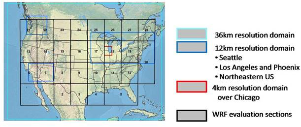
Figure 1. Nested model domains (36, 12, and 4 km domains) overlaid by 28 evaluation blocks for
characterization of meteorological error.
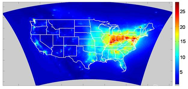
Figure 2. PM2.5 simulation result, annual average PM2.5 for 2002. Coor scale is PM2.5 in µg m-3.
| Season | Number Pairs | Model Mean PM2.5 (µg/m3) | OBS Mean PM2.5 (µg/m3) | Mean Bias (µg/m3) | Mean Error (µg/m3) | Mean Fractional Bias | Mean Franctional Error | Correlation Coefficient (r) |
|---|---|---|---|---|---|---|---|---|
| CONUS 36 km parent domain | ||||||||
| Spring | 14374 | 12.3 | 11.0 | 1.3 | 6.0 | -4 | 53 | 0.47 |
| Summer | 16860 | 11.2 | 16.1 | -4.8 | 7.7 | -4.5 | 62 | 0.50 |
| Fall | 15393 | 15.3 | 11.7 | 3.5 | 7.7 | 12 | 57 | 0.54 |
| Winter | 13332 | 14.3 | 11.6 | 5.7 | 8.6 | 30 | 58 | 0.56 |
| Northeaster U.S. 12 km subdomain | ||||||||
| Spring | 6757 | 15.4 | 11.3 | 4.2 | 5.9 | 21 | 43 | 0.69 |
| Summer | 7040 | 16.0 | 18.4 | -2.4 | 7.2 | -16 | 45 | 0.56 |
| Fall | 7476 | 18.9 | 11.8 | 7.1 | 8.3 | 39 | 52 | 0.69 |
| Winter | 6317 | 23.8 | 12.8 | 11.0 | 11.7 | 57 | 63 | 0.68 |
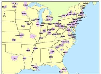
Figure 3. Geographical boundaries (MSAs and other) used in earlier
analysis of PM2.5 vs. the American Cancer Society (ACS) cohort.
Western MSA boundaries are not shown in this figure.
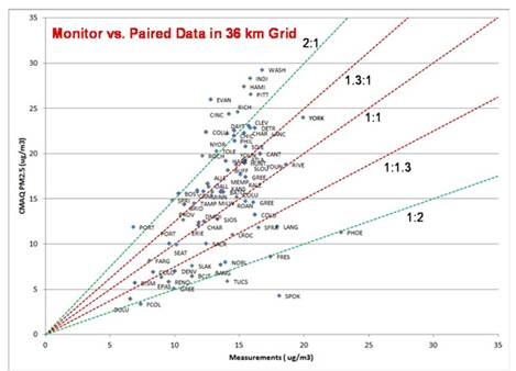
Figure 4. Measured PM2.5 and modeled PM2.5 restricted to ACS MSAs.
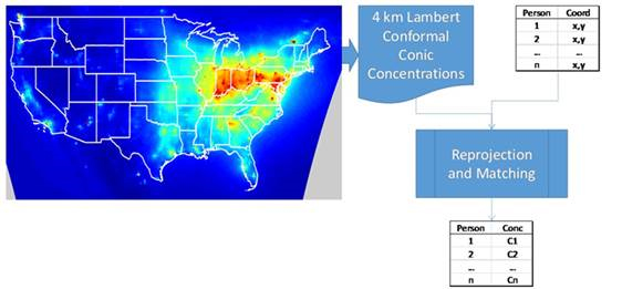
Figure 5. Flowchart showing the matching of concentrations to the individuals in the epidemiological cohort.
Based on coordinates of the individuals (count n) in the cohort, each person is assigned a consternation C1 through Cn.
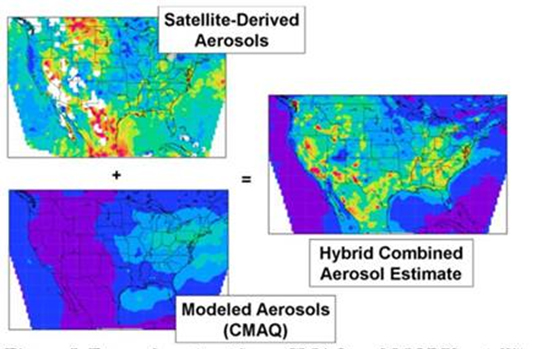
Figure 6. Example output from CMAQ and MODIS sattellite (regridded to CMAQ domain) for
January 2002. Combinationof these using optical interpolation leads to the hybrid values shown
on the right.
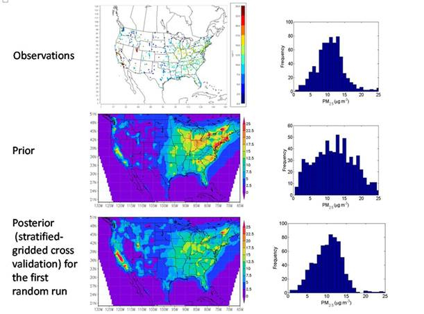
Figure 7. Example of surface measurement data assimilation for January 2002. Top row are measurement
values for PM2.5, assigned to the CMAQ grid as a map (left) and histogram (right). Middle row are
CMAQ model values before assimilation as a map (left) and as a histogram (right). Bottom row is the
posterior PM2.5 using optimal interpolation to sombine the first two rows.
| Grouping | Sources |
|---|---|
| Liquid Fuels Combustion | Onroad diesel vehicles (L1) |
| Nonroad diesel engines (L2) | Onroad gasoline vehicels (L3) Nonroad |
| Gasoline engines (L4) | Oil cumbustion (L5-LEGU, L5-nLEGU) |
| Gaseous Fuels Combustion | Natural gas (G-EGU, C1-nEGU) |
| Coal combustion | Coal combustion (C1 -EGU, C1-nEGU) |
| Biomass Burning | Agricultural burning (B1) fireplace/woodstove (B2) |
| Residential yard and solid waste burning (B3) Wildfires (B4) | Prescribed burning (B5) |
| Dust | Road dust (D1) |
| Unpaved road dust (D2) | Other fugitive dust (D3) |
| Industrial sources | Pulp, paper and wood process i ng (P1) |
| Primary metal processes (P2 | |
| Mineral industrial processes (P3) | Other industrial processes (P4) |
| Other | Other fuel combustion (O1) other (02) |
Figure 8. Example of source-resolved emissions input to CMAQ. Nonroad diesel engines PM2.5 emissions. Left shows linear scale,
emphasizing major metropolitan areas. RIght shows log scale, demonstrating that emissions are included in the model for all of the
U.S. and Canada.
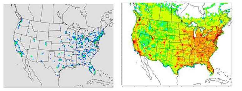
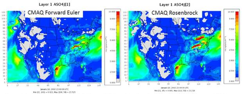
Figure 9. Comparison of sulfate predictions for the standard CMAQ forward Euler method (left) and the University of Iowa CMAQ/Rosenbrock solver (right)
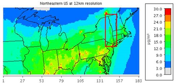
Figure 10. PM2.5 in the Northeastern U.S. 12 km domain. Red box shows the Hudson RIver valley,
which has an increment over the surrounding rural areas when simulated at 12 km, but not at 36 km.
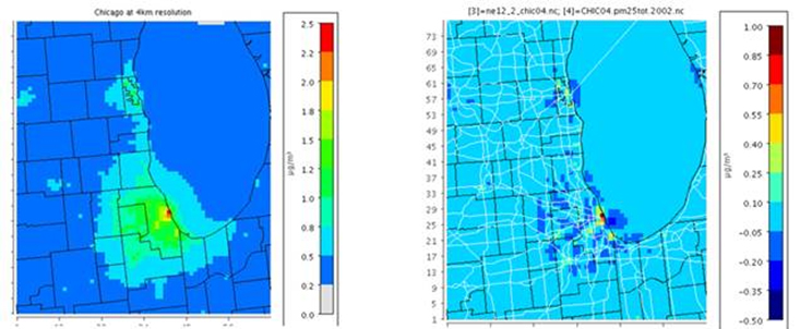
Figure 11. 4-km Elemental Carbon (EC) in the Chicago 4-km domain. Left panel shows annual average 4-km EC. Right panel
shows difference between the 12-lm simulation and 4-km simulation. Concentrations in the city center are increased at high
resolution, and decreased in the margins within ~12 km of the high emission grid cells.
| Season | Number Pairs | Model Mean PM2.5 (µg/m3) | OBS Mean PM2.5 (µg/m3) | Mean Bias (µg/m3) | Mean Error (µg/m3) | Mean Fractional Bias | Mean Franctional Error | Correlation Coefficient (r) |
|---|---|---|---|---|---|---|---|---|
| Chicago model vs. obervation at 12-km | ||||||||
| Spring | 446 | 13.5 | 11.1 | 2.4 | 4.0 | 15 | 32 | 0.73 |
| Summer | 388 | 13.9 | 15.3 | -1.5 | 4.1 | -10 | 30 | 0.75 |
| Fall | 412 | 19.2 | 13.5 | 5.7 | 6.9 | 33 | 41 | 0.80 |
| Winter | 424 | 19.0 | 13.6 | 5.5 | 6.8 | 37 | 45 | 0.47 |
| 4 km | ||||||||
| Spring | 445 | 14.8 | 11.1 | 3.6 | 5.1 | 21 | 37 | 0.66 |
| Summer | 388 | 14.6 | 15.3 | -0.7 | 4.6 | -7 | 32 | 0.66 |
| Fall | 412 | 19.8 | 13.5 | 6.2 | 7.4 | 34 | 43 | 0.80 |
| Winter | 424 | 19.8 | 13.6 | 6.02 | 7.6 | 40 | 47 | 0.38 |
| Quesstions of Objective | Result |
|---|---|
| To create a database of PM2.5 concentratins for studying data assimilation techniques, best modeling practices (for health studies), and links to epidemiology. | We have completed continual CMAQ modeling for 2001 and 2002 using a combination of 36, 12, and 4 km domains. Other years and sorce-resolved model results (target year for them is 2002) are incomplete as of 6/1/2014 |
| Feasibility of linking to a large epidemiology cohort. | Our domains have been linked to the ACS cohort (200,000 + mortality cases) and preliminary calculations of relative risk to modeled PM2.5 were calculated. |
| How good is modeled PM2.5 for use in long-term epidemiologial studies such as with the ACS corhort? | High PM2.5 model error and spatial structure in bias are problematic for their use in an epidemiological study - improvements via data assimiliation or regression calibration are needed; Comparing PM2.5 concentrations in the model versus measured values in teh ACS cohort shows that a majority of the areas are predicted to within a 2:1 envelope, but model overprediction is somewhat severe in locaitons (mostly in the Midwestern U.S. |
| What are some of the promising data assimilation techniques? | Optimal interpolation of surface observations has been shown to substantially reduce bias and error relative to witheld data. |
| What about data assimilation of satellite data? | Methods explored in this project are not as successful as optimal interpolation of the surface measurements, although more effective alternate methodologies cannot be ruled out. |
| What are some of the issues with using MODIS aerosol optical depth? | MODIS bias and error combined with variable model bias make the problem difficult. |
| What degree of improvement can be achieved using the MODIS aeorsol optical depth and method of this work? | The best combinations of setting/schemes led to a domain average improvement in franctional error from 0.72 to 0.58 at IMPROVE monitoring sites, and from 0.59 to 0.53 at STN monitoring sites; somewhat larger improvements to fractional bias were observed; for 39% of the month-region combinations, no settings lead to improvement via OL. |
| Which is more important, positive bias of MODIS in teh Western U.S., or negative bias of CMAQ in the Western U.S. for windblown dust? | MODIS AOD positive bias (in the west) were more important than negative bias in CMAQ for coarse aerosols (i.e., wind-blown dust) |
| What are some recommendations for improving results from assimilation of satellite AOD? | REcommendations: use of improved MODIS retrievals are proposed in collection 6, and the integratin of AOD from both MISR and MODIS. |
| How does model preformance for total PM2.5 change between 12 km and 4 km resolution? | For our WRF3.3.1 configuration performance somtimes inproved with finer resolution, but not always. |
| What is the progress toward development of the adjoint of CMAQ and target-oriented sensitivities. | Progress of the adjoint of CMAQ continues within multiple research groups; efforts within project to replace the default CMAQ 4.7.1 aqueous chemistry routine with a version based on the Kinetic PreProcessor (KPP) that would promote efficient calculation of the model adjoint were initially promising, but numerical issues have not yet been fully addressed. |
The proposal called for application of a 3D chemical transport model with an adjoint model (including gas, transport, and aerosol processes). This was a necessary component to the demonstration of target oriented sensitivity calculations. We chose to join a CMAQ adjoint development group, led by Amir Hakami and Daven Henze, in 2010. The initial thinking was that a community adjoint model could be completed in about two years; however, four years into the project, a CMAQ adjoint modeling system suitable for the project goals is not yet available.
| Vriable | Setting (wrf namelist settings in parenthesis) |
|---|---|
| Nesting | one way nesting |
| Vertical Resolution | 30 levels First layer depth -20m Model top 100 mbar |
| Spinup period | 24 h |
| Run time before initialization (excluding spinup) | 150 hrs |
| Land cover | USGS 24-category Land Use Categories |
| Treatment of Snow (albedo, incluence on surface engery and moisture balance) | 1 |
| Initial and Boundary Conditions | NARR |
| isffix & icloud | 1 |
| Data assimiliation to improve initial boundary conditions via objective analysis (OBSGRID), e.g. making metos_em* files instead of met_em* | yes |
| Data souce for Objective Analysis | ADP surface and upper measurements |
| Obervation nudging - is it used (i.e. obs_msdge_opt | NO - analysis and surface nudging used, but not observational nudging |
| Grid (analysis) nudging via FDDA. Settings above surface layer (grid_fdda) | Nudge temperature and humidity and winds through entire depth u.v: 5x10⁻⁴ (36 km), 3x10⁻⁴ (12 and 4 km) T: 5x10⁻⁴ (36 km), 3x10⁻⁴ (12 and 4 km) q: 1x10⁻⁵ (36, 12 & 4 km) nudging at 3 hr intervals |
| Grid (surface) nudging in the surface layer (grid_sfdda) [Yes/No + data source) | Yes on 12 km and 4 km - OBSGRID run on METAR files to generate ndtedf files for surface |
| Settings for SFDDA settinss at surface (grid_sfdda settings) | Nudge winds at surface 5x10⁻⁴ nudging at 3 hr intervals |
| PBL Scheme (bl_pbd_physics) | ACM2(7) |
| Microphysics scheme (mp_physics) | Morrison (10) |
| Radiation scheme (ra_lw_phusics, ra_sw_physics) | RRTMG(4), SQ and LW time steps 12 min, 4 min and 1 min |
| Land surface scheme (sf_sfclay_physics and sf_surface_physics) | Pleim-Xiu(7) |
| Cumulus scheme (cu_physics) | Kain-Fritsch(1) |
| Soil moisture treatment/soil layers | default 2 layers |
| Tiime step | 120 sec at 35 km; 40 sec at 12 km & 10 sec at 4 km |
| Dynamics damping (w_dumping, damp_opt) | w_damping = 1 damp_opt = 3 |
| Modeling Year | NEI Year | On-road source | Non road source | Point source | CEM | Area source | Canada |
|---|---|---|---|---|---|---|---|
| 2000 | 2001 | Projected using EGAS 4.0 VMT | 2001 | Projected using EGAS 4.0 | 2000 | 2001 | * |
| 2001 | 2001 | 2001 | 2001 | 2001 | 2001 | 2001 | * |
| 2002 | 2002 | 2002 | 2002 | 2002 | 2002 | 2002 | * |
| 2003 | 2002 | Projectied using EGAS 4.0 VMT | 2002 | Projectied using EGAS 4.0 VMT | 2003 | 2002 | * |
| 2004 | 2005 | Projectied using EGAS 4.0 VMT | 2005 | Projectied using EGAS 4.0 VMT | 2004 | 2005 | * |
| * Area, nonroad and mobile emission rates are linearly interpolated using 2000 and 2010 data. 2006 Point source data was projected back to the simulation year using Canada emission trends. Overall pollutant scaling factors are applied. | |||||||
Details of methods selection and results for satellite data assimilation are attached as Appendix 2. Appendix 3 contains methodological details and results for data assimilation of surface PM2.5 measurements.
Efforts towards development of the adjoint model of CMAQ
Details of methods and results for our development work regarding a new version of the CMAQ module AQCHEM using the Kinetics Preprocessor (KPP) tool with automatic generation of adjoint code can be found in Appendix 4.
Conclusions:
Progress has been made in all of these goals, but progress to date unfortunately remains short of our proposed outcomes. As the formal grant period is over, we are summarizing progress and outcomes to date in this report; however, we continue to work to achieve a greater fraction of the proposed goals and publish more manuscripts on the work related to our EPA grant. We will notify EPA of additional publications resulting from this project as they are accepted. Reasons for the incomplete objectives are discussed in the report.
References:
Journal Articles on this Report : 9 Displayed | Download in RIS Format
| Other project views: | All 26 publications | 9 publications in selected types | All 9 journal articles |
|---|
| Type | Citation | ||
|---|---|---|---|
|
|
Baxter LK, Dionisio KL, Burke J, Sarnat SE, Sarnat JA, Hodas N, Rich DQ, Turpin BJ, Jones RR, Mannshardt E, Kumar N, Beevers SD, Ozkaynak H. Exposure prediction approaches used in air pollution epidemiology studies: key findings and future recommendations. Journal of Exposure Science & Environmental Epidemiology 2013;23(6):654-659. |
R833865 (Final) R834799 (2014) R834799 (2015) R834799 (2016) R834799 (Final) R834799C004 (2013) R834799C004 (2014) R834799C004 (2015) R834799C004 (Final) |
Exit Exit Exit |
|
|
Fahey KM, Carlton AG, Pye HOT, Baek J, Hutzell WT, Stanier CO, Baker KR, Appel KW, Jaoui M, Offenberg JH. A framework for expanding aqueous chemistry in the Community Multiscale Air Quality (CMAQ) model version 5.1. Geoscientific Model Development 2017;10(4):1587-1605. |
R833865 (Final) R835041 (Final) |
Exit Exit |
|
|
Kumar N, Chu AD, Foster AD, Peters T, Willis R. Satellite remote sensing for developing time and space resolved estimates of ambient particulate in Cleveland, OH. Aerosol Science and Technology 2011;45(9):1090-1108. |
R833865 (Final) R835193 (Final) |
Exit Exit |
|
|
Liang D, Kumar N. Time-space Kriging to address the spatiotemporal misalignment in the large datasets. Atmospheric Environment 2013;72:60-69. |
R833865 (Final) |
Exit Exit Exit |
|
|
Porter AT, Oleson JJ, Stanier CO. On the spatio-temporal relationship between MODIS AOD and PM2.5 particulate matter measurements. Journal of Data Science 2014;12(2):255-275. |
R833865 (2012) R833865 (Final) |
Exit Exit |
|
|
Zhang HL, Ying Q. Secondary organic aerosol from polycyclic aromatic hydrocarbons in Southeast Texas. Atmospheric Environment 2012;55:279-287. |
R833865 (Final) |
Exit Exit Exit |
|
|
Zhang HL, Zhang HL, Li JY, Ying Q, Guven BB, Olaguer EP. Source apportionment of formaldehyde during TexAQS 2006 using a source-oriented chemical transport model. Journal of Geophysical Research-Atmospheres 2013;118(3):1525-1535. |
R833865 (Final) |
Exit Exit |
|
|
Zhang H, Li J, Ying Q, Yu JZ, Wu D, Chen Y, He K, Jiang J. Source apportionment of PM2.5 nitrate and sulfate in China using a source-oriented chemical transport model. Atmospheric Environment 2012;62:228-242. |
R833865 (Final) R833864 (2011) R833864 (2012) R833864 (2013) R833864 (Final) |
Exit Exit Exit |
|
|
Zhang H, Chen G, Hu J, Chen S-H, Wiedinmyer C, Kleeman M, Ying Q. Evaluation of a seven-year air quality simulation using the Weather Research and Forecasting (WRF)/Community Multiscale Air Quality (CMAQ) models in the eastern United States. Science of the Total Environment 2014;473-474:275-285. |
R833865 (Final) R833864 (2013) R833864 (Final) |
Exit Exit Exit |
Supplemental Keywords:
Air, health effects, human health, modelingProgress and Final Reports:
Original AbstractThe perspectives, information and conclusions conveyed in research project abstracts, progress reports, final reports, journal abstracts and journal publications convey the viewpoints of the principal investigator and may not represent the views and policies of ORD and EPA. Conclusions drawn by the principal investigators have not been reviewed by the Agency.