
Grantee Research Project Results
2011 Progress Report: Consequences of Global Climate Change for Stream Biodiversity and Implications for theApplication and Interpretation of Biological Indicators of Aquatic Ecosystem Condition
EPA Grant Number: R834186Title: Consequences of Global Climate Change for Stream Biodiversity and Implications for theApplication and Interpretation of Biological Indicators of Aquatic Ecosystem Condition
Investigators: Hawkins, Charles P. , Tarboton, David G. , Jin, Jiming
Institution: Utah State University
EPA Project Officer: Packard, Benjamin H
Project Period: September 1, 2009 through August 31, 2012 (Extended to July 31, 2013)
Project Period Covered by this Report: September 1, 2010 through August 31,2011
Project Amount: $789,532
RFA: Consequences of Global Change for Water Quality (2008) RFA Text | Recipients Lists
Research Category: Aquatic Ecosystems , Ecological Indicators/Assessment/Restoration , Watersheds , Water , Climate Change
Objective:
The main objective of our proposed research is to assess how changes in stream temperature and hydrology associated with global/regional climate change will influence (1) site- and regional-scale biodiversity of stream ecosystems and (2) the performance and interpretation of biological indicators, which are used to determine if streams are meeting the biological water quality goals of the Clean Water Act.
Progress Summary:
Our main accomplishments since the previous progress report of July 23, 2011, include: (1) expansion of three stream temperature models initially developed for the United States west of the Mississippi River to the CONUS, (2) application of these stream temperature models to historical early 20th century and forecast 21st century climate regimes to quantify how stream thermal regimes have changed and will continue changing with climate change, (3) refinement of candidate stream flow variables to better characterize the main components of the flow regime and calculation of these variables at 1512 reference-quality USGS gauging stations, (4) analysis of historical trends in precipitation and stream flow variables, and (5) characterization and mapping of major stream flow regimes within the CONUS under existing climate regimes.
As reported in July 2011, we used Random Forests (RF) to empirically model stream temperatures (STs) across a range of stream and river sizes and landscape settings within the western United States. These models were developed with USGS temperature stations that were determined to be in reference condition and for three seasonal periods: mean daily summer (July-August), winter (January-February), and annual stream temperatures (MSST, MWST, and MAST, respectively).
We expanded these models to include USGS stations across the CONUS. We selected ST stations in reference condition following the methods outlined in the previous progress report. Reference screening resulted in 507 summer, 657 winter, and 238 annual USGS stations considered to be in reference condition. Each station has 1 – 10 years of temperature record, and therefore resulted in 1635 summer, 2819 winter, and 871 annual ST observations. We used GIS-derived information about the climate of each year of ST record (air temperature), and time-invariant factors such as topography, watershed area, and soils at each station to develop RF models of ST for the CONUS. Both internal RF and external validations of the models suggest excellent performances (Table 1).
| Table 1. Internal and external (50 stations withheld) validation of reference condition ST models. | ||||
| Internal RF validation | External validation | |||
| Model | Pseudo-R2 | RMSE (°C) | r2 | RMSE (°C) |
| Summer | 0.97 | 1.1 | 0.92 | 1.9 |
| Winter | 0.97 | 0.75 | 0.91 | 1.4 |
| Annual | 0.98 | 0.67 | 0.94 | 1.2 |
We used these models to investigate how climate change has affected STs over the last century and will continue to do so over the next century. Long-term historical records of ST are rare, and empirical modeling will therefore be an important tool to understanding these impacts. We validated the use of these models to track the effects of climate change on STs by applying the models to the earliest ST records that were available (1976-1980). Time-series plots of air temperature, and observed and predicted MSSTs suggest that the models are successful in predicting changes in STs due to climate change (Fig. 1). We applied the models to historical (PRISM) air temperatures during the period of 1900-1909. Hindcasting results suggest that CONUS MSSTs, MWSTs, and MASTs have respectively risen by 0.4, 0.5, and 0.2 °C over the last century on average. In addition, we applied a downscaled A2 GCM climate forecast (years 2090-2099) to the MSST model. Forecasting results suggest that MSSTs could warm by an additional 0.65 °C on average by the end of the 21st century. However, sensitivities of individual streams varied greatly to climate changes (Fig. 2).
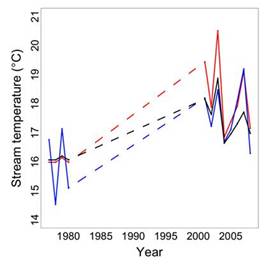
Fig. 1. An example time-series plot of observed PRISM air temperature (red), and observed (blue) and predicted (black) STs at a USGS gauge station.
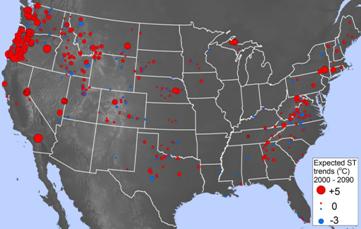
Fig. 2. Distribution of projected MSST warming (red) and cooling (blue) at reference condition USGS stations. Symbol sizes are proportional to the expected magnitude of change. The average stream temperature change from 2000-2090 is expected to be +0.65 °C.
Future Activities:
Ongoing and future work: Understanding the differential sensitivity of streams to climate change will be important when designing mitigation efforts. We are investigating the watershed and stream attributes that are associated with greater sensitivities to shifting climates. We used RFs to model the differences between current and predicted future MSSTs (R2 = 0.62). The model suggested that larger air temperature shifts, cooler initial stream temperatures, and smaller channel slopes were all associated with more sensitive MSSTs. Intermediate levels of both catchment relief and area were associated with less sensitive MSSTs. This modeling approach will be applied to MWSTs and MASTs to understand their potential differing sensitivities as well. These results will be presented at the national meeting of the Society for Freshwater Science in Louisville, KY, in May 2012. A manuscript of this work is expected to be submitted for publication within the next 2 months. In addition, the RF models will be used to produce estimates of the current and future thermal regimes for a network of 1000s of stream sites for which biotic samples have been taken. These data will be used in the next phase of the project to understand the potential effects of climate change, and the associated alterations in STs, on the biodiversity of the Nation’s streams.
Our previous work identified 17 candidate flow variables that characterize the flow regimes of streams and river within the CONUS. In addition to these 17 variables, we also developed an index of flow steadiness. We developed the steadiness index (SI) because subsequent analyses required that variables be normally distributed. However, two of the 17 candidate variables (base flow index [BFI] and zero flow days [ZD]) could not be transformed to meet this assumption because of numerous zero values present within both. We combined BFI and ZD to produce the SI based on the following logic: (1) when ZD = 0 (i.e., water is flowing) and therefore non-informative, BFI describes low flows near zero; and (2) when ZD > 0, and thus describing the duration of no flow, BFI = 0 and non-informative (Fig. 3). By combining BFI and ZD, we produced a new variable (SI) that is informative of both no- and low-flow conditions and can be transformed to be normally distributed. SI is calculated as the difference between BFI and ZD after rescaling each predictor from 0 to 1 and -1 to 0, respectively (Fig 3). We have calculated these flow variables for 1512 reference-quality USGS gauging stations distributed across the CONUS with long-term flow data.
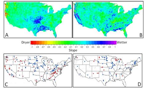
We investigated the historical spatial trends in precipitation by developing time-series quantile regressions for each PRISM climate pixel, i.e., an individual time-series regression model for each 4-Km cell within the map. The slope of each quantile regression was mapped and allowed us to visualize trends in low (20% quantile) and high (80% quantile) monthly precipitation over from 1949 to 1999. In addition to trends in precipitation, we developed time-series regressions for each of the flow variables at each station during their respective periods of record. Comparing maps of the trends suggests that regions that are becoming wetter (positive 20% and 80% quantile regression slopes) have increased BFI values and mean daily flows, respectively (Fig. 4).
Fig. 3. The cumulative probablity distributions of ZD (A) and BFI (B). SI (C) is a combination of both ZD and BFI.
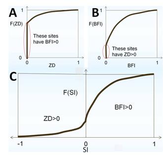
Fig. 4. Mapped slopes of the 20% (A) and 80% (B) PRISM climate time-series quantile regressions. Significant (p < 0.01) positive (blue) and negative (red) linear regression trends in BFI (C) and mean daily flow (D).
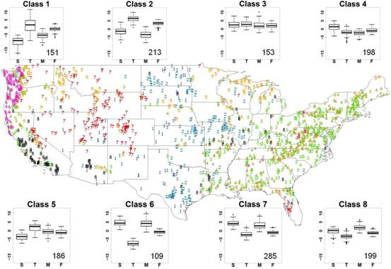
To characterize the main components of flow within the CONUS, we then applied a Principal Components Analysis (PCA) to the 16 flow variables to reduce the dimensionality of the data to four main axes of flow: (1) steadiness, (2) timing, (3) magnitude, and (4) flood duration (Table 2). We used the PCA axis scores in a K-means clustering to classify the 1512 USGS stations into flow regime types. A range of class sizes were used (K = 4 to 8 groups), and these classes were mapped to identify regions of similar flow regime (Fig. 5).
Fig. 5. An example of the spatial distribution of sites within 8 flow regime classes (K = 8). Box plots show the distribution of the varimax-rotated PCA axis scores across the 8 classes. The letters represent the 4 main flow axes that were identified with the PCA: steadiness (S), timing (T), magnitude (M), and flood duration (F). The number of USGS stations within each class is displayed at the bottom-right of each box plot.
| Variable | Axis 1 | Axis 2 | Axis 3 | Axis 4 |
|---|---|---|---|---|
| SI | 0.793 | 0.144 | 0.098 | 0.242 |
| Coefficient of variation of daily flow | -0.850 | -0.002 | -0.064 | -0.340 |
| Mean daily discharge | 0.342 | -0.104 | 0.923 | 0.068 |
| Flow with a 1.67 year recurrence interval | 0.061 | -0.169 | 0.963 | -0.176 |
| Flood duration | -0.107 | 0.387 | -0.089 | 0.747 |
| Average 7 day minimum flow | 0.739 | 0.073 | 0.557 | 0.186 |
| Average 7 day maximum flow | 0.097 | -0.107 | 0.985 | -0.009 |
| Flow reversals per year | 0.673 | -0.118 | 0.254 | -0.383 |
| Colwell’s index of predictability | -0.783 | 0.231 | -0.092 | 0.341 |
| Colwell’s index of constancy | -0.836 | 0.251 | -0.104 | -0.055 |
| Colwell’s index of contingency | 0.369 | -0.072 | 0.033 | 0.771 |
| Day of year by 25% of total flow has occurred | -0.417 | 0.777 | -0.083 | 0.278 |
| Day of year by 50% of total flow has occurred | -0.065 | 0.945 | -0.091 | 0.186 |
| Day of year by 75% of total flow has occurred | 0.204 | 0.918 | -0.080 | 0.024 |
| Day of year of peak flow | -0.032 | 0.775 | -0.096 | -0.102 |
| Day of year of peak of a sine function fit to flow | -0.168 | 0.853 | -0.073 | 0.127 |
| Interpretation % of variance explained by axis | Steadiness 26 | Timing 25 | Magnitude 20 | Flood Duration 21 |
Ongoing and future work: We are working to develop empirical relationships between the flow variables and hydrologic regime classes with climate (precipitation and temperature) and time-invariant watershed features such as topography, watershed area, and soils to enable their prediction to ungauged streams. In addition, we will apply these empirical relationships to downscaled climate forecasts to explore how the hydrologic regime will respond to climate changes over the 21st century. Finally, the forecasted changes in hydrologic regime will be used to explore their potential effects on biodiversity across the CONUS.
Modeling expected ecological impacts of climate change
This aspect of the modeling cannot proceed until the climate and hydrologic modeling is complete. We anticipate initiating the baseline models starting this summer.
Journal Articles on this Report : 5 Displayed | Download in RIS Format
| Other project views: | All 73 publications | 14 publications in selected types | All 12 journal articles |
|---|
| Type | Citation | ||
|---|---|---|---|
|
|
Hill RA, Hawkins CP, Carlisle DM. Predicting thermal reference conditions for USA streams and rivers. Freshwater Science 2013;32(1):39-55. |
R834186 (2011) R834186 (2012) R834186 (Final) |
Exit Exit Exit |
|
|
Jin J, Miller NL. Improvement of snowpack simulations in a regional climate model. Hydrological Processes 2011;25(14):2202-2210. |
R834186 (2010) R834186 (2011) R834186 (2012) R834186 (Final) |
Exit Exit |
|
|
Jin J, Miller NL. Regional simulations to quantify land use change and irrigation impacts on hydroclimate in the California Central Valley. Theoretical and Applied Climatology 2011;104(3-4):429-442. |
R834186 (2010) R834186 (2011) R834186 (2012) R834186 (Final) |
Exit Exit Exit |
|
|
Jin J, Wen L. Evaluation of snowmelt simulation in the Weather Research and Forecasting model. Journal of Geophysical Research-Atmospheres 2012;117(D10):D10110 (16 pp.). |
R834186 (2011) R834186 (2012) R834186 (Final) |
Exit Exit Exit |
|
|
Zhao L, Jin J, Wang S-Y, Ek MB. Integration of remote-sensing data with WRF to improve lake-effect precipitation simulations over the Great Lakes region. Journal of Geophysical Research-Atmospheres 2012;117(D9):D09102 (12 pp.). |
R834186 (2011) R834186 (2012) R834186 (Final) |
Exit Exit Exit |
Supplemental Keywords:
PA Regions 1-10, thermal modification, hydrologic modification, modeling, biological indicators, biological assessment, biological integrity, air, RFA, climate change, air pollution effects, atmosphere;, RFA, Air, Atmosphere, Air Pollution Effects, climate changeProgress and Final Reports:
Original AbstractThe perspectives, information and conclusions conveyed in research project abstracts, progress reports, final reports, journal abstracts and journal publications convey the viewpoints of the principal investigator and may not represent the views and policies of ORD and EPA. Conclusions drawn by the principal investigators have not been reviewed by the Agency.