
Grantee Research Project Results
2008 Progress Report: Regional Development, Population Trend, and Technology Change Impacts on Future Air Pollution Emissions in the San Joaquin Valley
EPA Grant Number: R831842Title: Regional Development, Population Trend, and Technology Change Impacts on Future Air Pollution Emissions in the San Joaquin Valley
Investigators: Kleeman, Michael J. , Niemeier, Deb , Lund, Jay , Handy, Susan
Current Investigators: Kleeman, Michael J. , Lund, Jay , Niemeier, Deb , Handy, Susan
Institution: University of California - Davis
EPA Project Officer: Chung, Serena
Project Period: October 1, 2004 through September 30, 2007 (Extended to September 30, 2010)
Project Period Covered by this Report: October 1, 2007 through September 30,2008
Project Amount: $680,000
RFA: Regional Development, Population Trend, and Technology Change Impacts on Future Air Pollution Emissions (2004) RFA Text | Recipients Lists
Research Category: Air , Climate Change
Objective:
The purpose of this study is to integrate economic forecasts with land-use models, water constraint models, travel demand models, and stationary source models to create an emissions modeling system that can be used to predict future air pollution emissions. The new emissions modeling system will be demonstrated by predicting air quality emissions in the San Joaquin Valley (SJV) in central California during the year 2030. Four objectives for the project are:
Objective 1: Create policy scenarios for the San Joaquin Valley (SJV) based on social and economic trends related to population growth, landuse policies, transportation investments, water availability, and energy technology. These scenarios will be used to drive the analysis for the remainder of the objectives. They should recommend the full range of possible futures for the valley, with emphasis on likely developments. Complete
Objective 2: Original: Predict future air quality emissions for the SJV using an integrated series of land use forecasting models, water-constraint models, travel demand models, on-road mobile source emissions models, non-road mobile source emissions models, and area source emissions models. Separate emissions inventories will be generated for each of the policy scenarios created during Objective 1. Revised: All of the original objectives are retained, and in addition to these we will study the influence of energy decisions on future air quality emissions in the SJV. The CA-TIMES energy model currently under development by researchers at the UC Davis Institute of Transportation Studies (ITS) will be used to predict changes in future emissions patterns for criteria pollutants related to energy production. In Progress
Objective 3: Transform the bulk emissions of volatile organic compounds (VOCs) and particulate matter (PM) listed in emissions inventories into composition resolved emissions of model species using “source profiles” measured during emissions tests. The resulting emissions inventories will be ready for model input. In Progress
Objective 4: Perform air quality simulations using the emissions inventories created in Objective 3 to evaluate the air quality implications of the policy scenarios created in Objective 1. This work will be combined with a project sponsored by the California Air Resources Board that seeks to predict how Climate Change will modify weather patterns at the urban and regional scale in California during the stagnation events that drive air quality episodes. In Progress
The objectives listed above are expanded relative to those described in our original proposal (see objective 2). The project is behind schedule but deliverables are being produced in step with project expenditures. The following statements summarize work status, work progress, preliminary data results, and evaluations during the reporting period.
Progress Summary:
September 2005
(1) UCD Develop initial list of variables that will affect air quality emissions. Completed. The project team selected an initial list of variables that were expected to influence future air quality emissions in SJV. Key policy variables were chosen based on two criteria: variables that can be represented in the modeling framework, and variables that reflect interesting or important possibilities for the San Joaquin Valley.
(2) UCD Background research into variables that will affect air quality emissions and preparation of white papers. Completed. The project team conducted background research into each key variable and determined the various policies proposed or already enforced for each variable. Several white papers were written for each variable. During the background research, the team also considered adding other variables that may impact future air quality emission. Global variables outside the San Joaquin Valley’s sphere of influence were acknowledged as influential on air quality, but were not extensively researched for the first phase of the project. Energy Costs/Availability was changed to encompass policies impacting temperature and energy. The variables Water Consumption Limits and Water Reuse were removed because it was determined by the team they are not determinate factors for growth and land use change. The overall water quantity available is the most important factor to consider. Thus, the variable Water Availability replaced these two variables because it would have a direct impact on land use allocation. Water Consumption Limits and Water Reuse will be considered in the water modeling phase of the project.
(3) UCD Creation of policy scenarios for air quality emissions in the San Joaquin Valley in 2030. Completed. The project team selected a limited number of values for each key variable. Generally, each variable was given values based on three possible levels: existing conditions, current trends, and maximum air quality benefits or growth minimized. Four initial scenarios were created based on a limited number of combinations of values of each of the policy variables: Baseline Scenario (assumes “no change” for all variables), Controlled Growth Scenario (assumes we do not expand roads, expand alternative forms of transportation, increase residential densities, and adopt all technologies to improve air quality), Uncontrolled Growth Scenario (assumes the opposite for each variable – we expand all roads, do not implement alternative forms of transportation, and do not adopt technologies to improve air quality) and the As Planned Scenario (represents what is currently planned as closely as possible). In this last scenario, there are both new roads and high speed rail, densities vary between low and high, and some technologies are adopted but they are not mandated.
(4) UCD Expert Panel meeting to review policy scenarios for air quality emissions in the San Joaquin Valley in 2030. Completed. An expert panel was assembled and a panel meeting was held to review the initial key variables, the values, and combinations of variables that formed a policy scenario. We assembled a panel of seven experts with diverse backgrounds in economics and land use, transportation, air quality, agriculture, and energy policy. The most important benefit from the expert panel was assistance in determining other possible variables impacting air quality and selecting the levels of variables that best represent the desired policy scenario outcome. After discussion with members from the expert panel, the team decided to add population as a global variable. Although policies will not necessarily impact population directly, there are a number of factors that will indirectly impact population such as economic factors, housing prices, etc. Therefore, we decided to vary this variable by 10 percent in either direction to account for possible changes in population. Other changes included adding buffers around freeways and certain land uses and a fuel tax as fixed assumptions.
(5) UCD UPLAN landuse modeling for initial policy scenarios. Completed. The UPLAN urban growth model is a rule-based grid model. It allocates the area of each land use type through a set of rules based on projected population increases, local land use plans, existing cities, and existing and planned transportation routes. Digital maps of current land use and zoning from the counties in the SJV were obtained and seven classes of land use were identified: Industrial, High Density Commercial, Low-Density Commercial, High-Density Residential, Medium-Density Residential, Low-Density Residential and Very-Low-Density Residential. Population growth estimates for the counties in the SJV were combined with information describing the location of cities, freeway ramps, highways, major arterials, minor arterials, vernal pools (a protected environmental feature) and flood plains to provide inputs for UPLAN estimates of future landuse. Each of the policy scenarios was evaluated separately to generate 4 initial patterns of landuse for each county in the SJV in the year 2030.
(6) UCD Travel demand modeling for the initial policy scenarios. Completed. Each of the 8 counties in the San Joaquin Valley has its own travel demand modeling system that integrates local information to estimate the number of trips between different locations using the commercial travel demand modeling package, TP+/Viper. All of the county-specific information was assembled by the UC Davis team and initial results were generated for the 4 preliminary policy scenarios. The “controlled” scenario with high-density land use pattern resulted in lower vehicle miles traveled (VMT) and vehicle hours traveled (VHT) at the regional level, as well as shorter travel distance and delay at the trip level. This indicates that people tend to travel less and make shorter trips under a condensed land use situation. Conversely, significant increases of VMT, VHT and average trip length are found in the “uncontrolled” scenario, due to highly sprawled land use patterns. The results in the “as planned” scenario are basically between that of the “controlled” and “uncontrolled” scenarios, suggesting some moderate increase of travel statistics than the baseline scenario.
September 2006
(7) STI Preparation of area-source and non-road mobile source inventories for the SJV in 2030. In progress. During 2005-06 STI reviewed the 2004 and ARB-projected 2020 “Almanac” emission inventories for the SJV to quickly identify the anticipated key sources of ROG, NOx, and PM in the SJV to help focus on the most significant emission sources. Key growth factors for CARB’s California Emission Forecasting System (CEFS) were provide for the key source categories to provide growth factors needed to project 2002 emissions in the SJV to 2030. CEFS does not include growth factors for most non-road mobile sources and so these were assembled separately using the methodology described by Puri and Kleinhenz, (1994) “A Study to Develop Projected Activity for Non-Road Mobile Categories in California, 1970-2020” with updated input information. Inputs and settings for CEFS and OFFROAD were customized to represent the conditions of the future-year scenarios selected by the UCD project team. Spatial allocation factors for area source and non-road mobile source emissions were developed using demographic and land use data from the UPLAN model and the latest spatial data sets.
During 2005-06, STI prepared approximations of one future-year emission inventory for areas of California outside the SJV. STI also provided technical support to UCD for issues related to geographic information systems (GIS). STI staff members attended periodic status and working meetings at UCD to discuss the project, review interim results, and formulate future-year scenarios of research interest for the SJV.
(8) STI Preparation of point source inventories for the SJV in 2030. In progress. The facility-specific emissions database available from ARB that lists annual emissions from 1995 – 2002. During 2004-05 the top 21 point sources (of 968 SJV facilities listed in the database) in 2002 were found to account for 33% to 55% of the ROG, NOx, and PM10 emissions. Updated forecasts for activity were compiled for industries relevant to the top 21 point sources including oil and gas extraction, cogeneration and refining. During 2005-06 STI prepared approximations of one future-year emissions inventory for point sources in California.
(9) Preparation of mobile source inventories for the SJV in 2030. In progress. During 2005-06 travel demand modeling was completed for the SJV. During 2005-06 one future year emissions inventory for mobile sources inside the SJV was prepared.
(10) Air Quality Modeling for the SJV in 2030. In progress. During 2005-06 one air quality model simulation was conducted using the available preliminary inventory.
September 2007
(7) STI Preparation of area-source and non-road mobile source inventories for the SJV in 2030. Complete. During 2006-07 STI completed preparation of area-source and non-road mobile source inventories for the 4 scenarios explored in the current project.
(8) STI Preparation of point source inventories for the SJV in 2030. Complete. During 2006-07 STI complete preparation of point-source inventories for the 4 scenarios explored in the current project.
(9) Preparation of mobile source inventories for the SJV in 2030. Complete. During 2006-07 mobile source inventories were completed for the 4 scenarios explored in the current project.
(10) Air Quality Modeling for the SJV in 2030. In progress. During 2006-07 emissions source profiles were developed for area and point sources that were not included in the standard profile library maintained by UCD. Several rounds of air quality simulations have been performed at various stages of emissions profile development. All simulations for the 2030 inventory should be finalized in the coming year.
September 2008
(11) Development of Emissions Inventories for Alternative Energy Policies in California in 2030. In Progress. A collaboration has been started between researchers in the current EPA project and the team of researchers building the CA-TIMES energy model which examines the impact of different energy policies on the demand and supply of energy in California. The spatial and temporal distribution of energy consumption produced in the landuse policy analysis will be retained for this portion of the project. The change in energy production by different sectors (hydro, natural gas, biomass, coal, …) will be used to scale the emissions of those sources relative to the basecase energy assumptions used in all of the current scenarios.
(12) Air Quality Modeling for the SJV in 2030. Complete for the original objectives and in progress for the revised objectives. The air quality simulations based on landuse policies in the SJV have been completed and the results are currently being analyzed in preparation for a series of publications. The air quality simulations based on energy policies in California will be completed when the energy policy emissions inventories are produced in Spring 2009.
Results During Preivious Year (Oct 2007 — Sept 2008)
Air Quality Model Emissions Preparation and Air Quality Model Results for Landuse Planning Scenarios
The four landuse future emissions scenarios were used to support air quality calculations for the state of California. A 190x190 grid domain was used along with California Regional Particulate Air Quality Study (CRPAQS) meteorology and boundary conditions representative of the time period December 15, 2000 – January 7, 2001. The four scenarios were then compared based on the variations in their emissions while under the same meteorological forcing. Calculations were performed at both 8km resolution and 4km resolution to help quantify potentially interesting effects related to population density. The current progress report focuses on the results generated with the highest resolution since lower resolutions have been discussed in previous reports and in meetings held with EPA.
Model simulations using 4km resolution were based on the four emissions scenarios generated by landuse policy decisions: Scenario 1 (baseline), Scenario 2 (controlled growth and reduced emissions), Scenario 3 (urban sprawl and no emissions controls), Scenario 4 (as planned growth and controls). Additional controls were applied to these initial emissions scenarios in the form of a residential, wood-burning ban. This control was deemed necessary across all scenarios as the additional organic carbon from the wood burning was pushing scenarios 1, 3 and 4 far beyond the current air quality standards and hence was not considered reasonable. Biogenic emissions were simulated for California using the emissions generation procedure provided by the California Air Resources Board as implemented on the UCD computing cluster. The biogenic emissions were scaled to approximate an average winter day based on temperature and shortwave radiation and based on landuse values for the year 2000 and 2001. The biogenic emissions were held constant between scenarios under the assumption that the majority of the biogenic emissions are released outside of the urban footprint associated with all scenarios. This assumption is appropriate since the majority of the photochemically relevant biogenic emissions in central California are associated with the areas around the edges of the SJV, not in the SJV.
Results are presented as the average hourly ambient conditions from December 25th to January 7th. Figure 1 shows the ambient PM2.5 organic carbon concentrations for Scenario 4 (as planned). PM2.5 OC hotspots in the SJV peak around the urban centers of Fresno (25 µg/m3) and Bakersfield (19 µg/m3). The other three scenarios look very similar to Scenario 4 when viewed at statewide-resolution and so results are presented as the difference between Scenario 4 and Scenario X.
Scenario 1 simulations predict a slight PM2.5 OC increase (~1 µg/m3) in the northern SJV with smaller ( < 0.5 µg/m3 ) decreases elsewhere (Figure 2). Scenario 2 (Figure 3) simulations predict increased OC concentrations around the urban centers (~2 µg/m3 ) and small decreases in rural areas ( < 0.5 µg/m3 ) . Since Scenario 2 contains more dense urban centers and sparser rural areas these results make sense when compared against Scenario 4. Scenario 3 (Figure 4) simulations predict enhanced OC concentrations in northern SJV (<2 µg/m3 ) and other rural areas showing a smaller increase ( < 0.5 µg/m3 ) with decreases around urban areas ( < 0.5 µg/m3 ). Again, these trends match the expected pattern since Scenario 3 allows the population to sprawl.
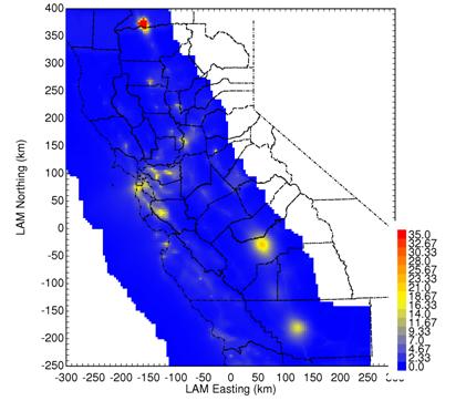
Figure 1: Organic Carbon PM2.5 two-week average hourly concentrations for Scenario 4.
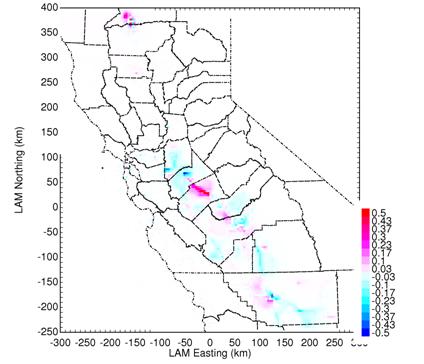
Figure 2: Organic Carbon PM2.5 two-week average hourly difference plot for Scenario 1 – Scenario 4.
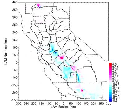
Figure 3: Organic Carbon PM2.5 two-week average hourly difference plot for Scenario 2 – Scenario 4.
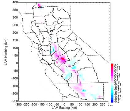
Figure 4: Organic Carbon PM2.5 two-week average hourly difference plot for Scenario 3 – Scenario 4.
The predicted differences in PM2.5 elemental carbon concentrations follow a similar pattern to those discussed for organic carbon above, but the absolute magnitude of the differences between scenarios is much smaller. Figure 5 shows the ambient elemental carbon present in PM2.5 for Scenario 4. The urban hotspots of Fresno and Bakersfield have EC concentrations that peak at approximately 5 µg/m3 while concentrations along major transportation corridors are closer to 2 µg/m3.
Figure 6 illustrates that PM2.5 EC concentrations predicted using Scenario 1 emissions change by less than 0.08 µg m-3 from Scenario 4 concentrations with the same spatial pattern noted for OC. Similarly, Scenario 2 follows the same pattern of urban increases and rural decreases discussed above, but with urban increases on the order of 0.08 µg/m3 and rural decreases on 0.08 µg/m3 (Figure 7). Scenario 3 again shows the converse of Scenario 2 with rural enhancement of EC around 0.09 µg/m3 and urban decreases up to 0.08 µg/m3 (Figure 8).

Figure 5: Elemental Carbon PM2.5 two week average hourly concentrations for Scenario 4.
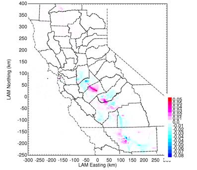
Figure 6: Elemental Carbon PM2.5 two week average hourly difference plot for Scenario 1 – Scenario 4.
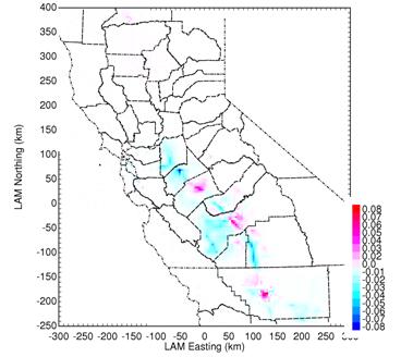
Figure 7: Elemental Carbon PM2.5 two week average hourly difference plot for Scenario 2 – Scenario 4.
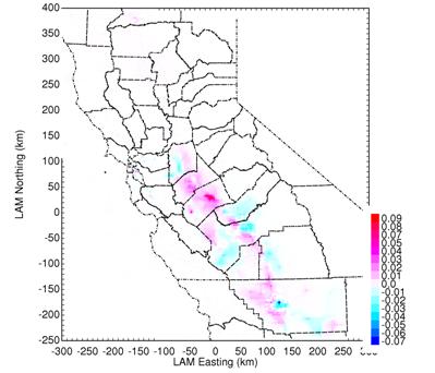
Figure 8: Elemental Carbon PM2.5 two week average hourly difference plot for Scenario 3 – Scenario 4.
Using the average ambient concentrations shown above with the population density maps for each scenario the average population weighted exposure was determined. Figure 9 illustrates the average population weighted exposure to PM2.5 organic carbon across the 2-week time period. Between the four scenarios the maximum average OC exposure is 5.48 µg/m3 for Scenario 2 and a minimum of 2.38 µg/m3 for Scenario 3. The error bars shown were calculated based on standard deviation of the average daily results from December 25th to January 7th. Scenario 2 and 3 do show a significant difference between their values. This difference is due to both the difference in ambient conditions as well as the differences in population density between the two scenarios.
It is noteworthy that Scenario 2 was initially designed to be the cleanest of the four scenarios under consideration. Scenario 2 has more emissions controls compared to the other scenarios but emissions are more concentrated in the urban areas due to landuse policies that encourage dense urban footprints. The urban population density in Scenario 2 is five times greater than the urban population density in Scenario 3. In the competition between the dilution vs. emissions controls, dilution appears to be the more important factor in the SJV. Predicted population-weighted exposures are higher for Scenario 2 than any other scenario studied.
Scenario 3 has fewer emissions controls compared to the other scenarios and emissions are more spread out across the region. While rural ambient concentrations are higher, overall the population isn’t as clustered in high pollution areas and exposure is lower on average.
The remaining scenarios do not appear significantly different based on the standard deviation.
The top 10th percentile exposure results (Figure 10) show that Scenario 2 has the highest exposure at 19.75 µg/m3 and Scenario 3 the lowest at 12.35 µg/m3. However, the results are not significantly different across any of the scenarios.
Figure 9: Average hourly population weighted exposure to organic carbon PM2.5.
Figure 10: 10th percentile hourly population weighted exposure to organic carbon PM2.5.
The population weighted results for elemental carbon following the same pattern as seen for organic carbon. Scenario 2 shows the highest average hourly exposure with 1.42 µg/m3 and the lowest exposure is Scenario 3 with 0.63 µg/m3 (Figure 11). These results appear to be significantly different using standard deviation to calculate the error. Scenarios 1 and 4 do not show a significant difference from the other scenarios.
There is no significant difference between the scenarios in the EC 10th percentile exposure results (Figure 12). The maximum exposure is 4.77 µg/m3 for Scenario 2 and the minimum is 3.28 µg/m3 for Scenario 3.
The results for elemental carbon and organic carbon components of PM2.5 point towards increased population exposure in the San Joaquin Valley for a controlled growth scenario even with a reduction in overall emissions. The urban sprawl scenario with uncontrolled growth and an overall increase in emissions resulted in lower exposure on average due to the population being sparser in the highest concentration areas. The 10th percentile numbers are less clear due in part to the high daily variability for each scenario
Figure 11: Average hourly population weighted exposure to elemental carbon PM2.5.
Figure 12: 10th percentile hourly population weighted exposure to elemental carbon PM2.5.
4.2 Air Quality Model Emissions Preparation and Air Quality Model Results for Alternative Energy Policy
Energy policy decisions in California will greatly influence future air quality emissions in the San Joaquin Valley. Researchers at the UC Davis Institute of Transportation Studies are in the process of analyzing future California energy pathways in support of greenhouse gas emissions studies. Dr. Sonia Yeh at ITS is developing the CA-TIMES energy model that will use energy policy constraints to determine the most economical way for California to satisfy its energy demand using a mix of potential energy sources. The current project will leverage this existing research to calculate changes to criteria pollutant emissions in response to different energy policies.
The output from the CA-TIMES energy model is divided into different categories: technologies, fuel use and greenhouse gas emissions. These categories will be mapped to the input parameters used to generate emissions of criteria pollutants for atmospheric chemistry calculations. The energy model generates hundreds of parameters based on sector, technology, equipment, fuel source, and equipment model year. The emissions generation system for criteria pollutants uses categories such as sector, industrial processes, equipment, fuel source and emission control equipment. The largest energy production categories identified in the CA-TIMES model will be mapped to equivalent criteria pollutant emissions categories. Changes to criteria pollutant emissions will be assumed proportional to energy output. The spatial distribution of all pollutant emissions will be based on the existing pattern of emissions sources under the assumption that any new facilities would be constructed at the same location as existing installations.
The Table below illustrates an example of mapping between the CA TIMES energy model and the criteria pollutant emissions model.
|
Technology
|
SSC #
|
ECI Description
|
|
Diesel Oil Combined-Cycle
|
20100102174
|
INTERNLCOMBUSTION ELECTRIC GENERATN DIST.OIL/DIESEL RECIPROCATING
|
|
|
20100301078
|
INTERNLCOMBUSTION ELECTRIC GENERATN DIESEL RECIPROCATING **
|
|
|
|
|
|
Diesel Oil Combustion Turbine
|
20100302116
|
INTERNLCOMBUSTION ELECTRIC GENERATN DIESEL TURBINE **
|
|
|
20100101174
|
INTERNLCOMBUSTION ELECTRIC GENERATN DIST.OIL/DIESEL TURBINE
|
|
|
|
|
|
Natural Gas Combined-Cycle
|
20100202080
|
INTERNLCOMBUSTION ELECTRIC GENERATN NATURAL GAS RECIPROCATING
|
|
|
|
|
|
Natural Gas Combustion Turbine
|
20100201080
|
INTERNLCOMBUSTION ELECTRIC GENERATN NATURAL GAS TURBINE
|
|
Oil Steam (Resid Fuel Oil LS)
|
31000411172
|
OIL & GAS PRODN FUEL-FIRED EQPMNT STEAM GENERATORS DISTILLATE OIL
|
|
|
31000412111
|
OIL & GAS PRODN FUEL-FIRED EQPMNT STEAM GENERATORS RESIDUAL OIL
|
|
|
31000413170
|
OIL & GAS PRODN FUEL-FIRED EQPMNT STEAM GENERATORS CRUDE OIL
|
Future Activities:
The final phase of the project will focus on refined air quality calculations based on the four emissions scenarios produced to date combined with the analysis of different energy pathways.
The preliminary air quality modeling results illustrated in Section 4 suggests some interesting trends in even the basecase growth scenario. Continued work will be done to identify the cause for each trend. The response of the future emissions system to emissions control programs will also be studied. Finally, population-weighted exposure to primary and secondary PM will be calculated under all scenarios.
Journal Articles:
No journal articles submitted with this report: View all 9 publications for this projectSupplemental Keywords:
RFA, Air, Scientific Discipline, Ecological Risk Assessment, Urban and Regional Planning, Atmosphere, Air Pollution Effects, climate change, Environmental Monitoring, air quality, ecosystem impacts, ecosystem models, Global Climate Change, economic models, climate variability, climate models, urban growth, human activities, demographics, emissions impact, land use, VOCs, atmospheric carbon dioxideProgress and Final Reports:
Original AbstractThe perspectives, information and conclusions conveyed in research project abstracts, progress reports, final reports, journal abstracts and journal publications convey the viewpoints of the principal investigator and may not represent the views and policies of ORD and EPA. Conclusions drawn by the principal investigators have not been reviewed by the Agency.