Grantee Research Project Results

Final Report: Consequences of Global Climate Change for Stream Biodiversity and Implications for theApplication and Interpretation of Biological Indicators of Aquatic Ecosystem Condition

EPA Grant Number: R834186
Title: Consequences of Global Climate Change for Stream Biodiversity and Implications for theApplication and Interpretation of Biological Indicators of Aquatic Ecosystem Condition
Investigators: Hawkins, Charles P. , Tarboton, David G. , Jin, Jiming
Institution: Utah State University
EPA Project Officer: Packard, Benjamin H
Project Period: September 1, 2009 through August 31, 2012 (Extended to July 31, 2013)
Project Amount: $789,532
RFA: Consequences of Global Change for Water Quality (2008) RFA Text | Recipients Lists
Research Category: Aquatic Ecosystems , Ecological Indicators/Assessment/Restoration , Watersheds , Water , Climate Change

Objective:

The main objective of our proposed research is to assess how changes in stream temperature and hydrology associated with global/regional climate change will influence (1) site- and regional-scale biodiversity of stream ecosystems, and (2) the performance and interpretation of biological indicators, which are used to determine if streams are meeting the biological water quality goals of the Clean Water Act.

Summary/Accomplishments (Outputs/Outcomes):

The challenge in assessing how stream biodiversity will respond to climate change involves linking several models that make realistic predictions about future climate change, stream temperature response to climate, stream flow response to climate, and invertebrate response to temperature and flow, respectively. We therefore developed downscaled climate models to predict future climate conditions, stream temperature and stream flow models that use climate conditions as predictors, and species distribution models (SDMs) that predict how the distributions of individual taxa and entire assemblages of taxa vary with stream temperature, flow, and other watershed attributes (Fig. 1). We describe each of these modeling efforts below.

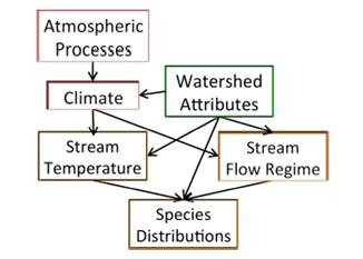
Figure 1. Conceptual diagram showing linkages between
atmospheric processes, climate, stream temperature,
flow regime, and species distribution models. Watershed
attributes are assumed to be time invariant but potentially
interact with climate sensitive processes.

Climate modeling – The main goal of the climate modeling was to produce reliable, high-resolution (4 km) climate simulations and forecasts for the contiguous United States (CONUS) for use in the hydrological and ecological analyses. To achieve this goal, we first calibrated and validated an advanced regional climate model (50 km resolution), the Weather Research and Forecasting (WRF) model, developed by the National Center for Atmospheric Research (NCAR) to ensure the model would generate realistic historical simulations – a necessary condition to have confidence in future climate predictions. During these evaluation processes, we ran the WRF model with observation-based reanalysis data to select the combination of physics schemes available in the model that produced optimal results. We also enhanced WRF model performance by coupling it to a sophisticated land surface model (the Community Land Model - CLM), which improved simulations of land surface processes that can influence climate. The NCAR WRF model development team has subsequently officially released this coupling work. The performance of regional models like WRF is also affected by the performance of the general circulation model (GCM) used to establish initial and lateral boundary conditions for the regional model. These GCM data often include significant biases resulting from the model’s coarse spatial resolution and oversimplified physics. We therefore needed to correct biases in the NCAR’s Community Climate System Model (CCSM) output (150 km resolution) before using it in our modeling. Biases in the CCSM output were minimized by regressing observed climate data on simulated (CCSM model) data and then adjusting CCSM predicted values based on these regression equations. The bias-corrected CCSM data were then used to drive the verified WRF model to produce 50 km climate simulations and forecasts for the CONUS. These 50 km resolution predictions were then further statistically downscaled to 4 km by regressing WRF output on 4 km resolution PRISM data for the CONUS. Below, we show that downscaling resulted in improved climate simulations and different forecasts than those associated with GCM forecasts.

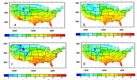
Temperature simulations for the period 1969-1999 based on different model configurations show how important downscaling and bias correction were in producing accurate forecasts (Fig. 2). Compared with PRISM 4 km observations (Fig. 2a), the coarse resolution CCSM simulations (Fig. 2b) were unable to accurately describe the spatial distribution of temperatures for the CONUS, especially for areas with complex terrain. Dynamically downscaling the CCSM simulations to 50 km resolution with the WRF model produced a better fit spatially between simulated and observed data (Fig. 2c). However, the WRF model produced cold biases over the high elevation areas in the West. The statistical downscaling to 4 km resolution produced simulations that were in very good agreement with the PRISM observations (Fig. 2d).

Figure 2. Temperature (°C) observations and simulations for the period of 1969 - 1999.
a) PRISM observations and 4 km resolution; b) the CCSM simulations at 150 km resolution;
c) WRF simulations at 50 km resolution forced with the biased corrected CCSM data; d) the
statistically downscaled WRF simulations at 4 km resolution.

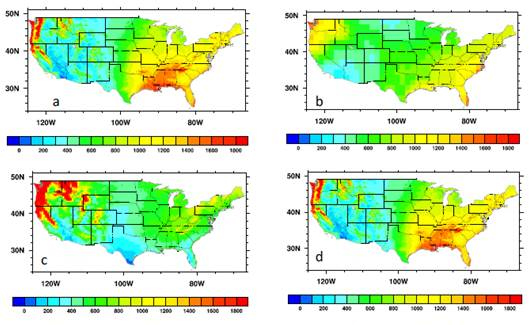
Precipitation simulations for the period 1969-1999 also showed how important downscaling and bias correction were in producing accurate forecasts (Fig. 3). Compared with PRISM observations (Fig. 3a), it is clear that strong orographically driven precipitation over the West Coast and in high elevation regions was not adequately represented in the CCSM simulations (Fig. 3b). In addition, the CCSM was unable to simulate high precipitation in the southeastern United States, which is mostly produced from tropical storms. The dynamically downscaled (50 km) WRF simulations better represented orographic precipitation over the West, but overestimated it (Fig. 3c). The WRF simulations also did not reproduce the high precipitation in the Southeast. Statistically downscaling precipitation to 4 km resolution (Fig. 3d) greatly improved the match between simulated and observed data across the entire CONUS.

Figure 3. Precipitation (mm/year) observation and simulations for the period 1969 - 1999. a)
PRISM observation at 4-km resolution; b) the CCSM simulations at 150-km resolution. c) WRF
simulations at 50-km resolution forced with the biased corrected CCSM data; d) the statistically
downscaled WRF simulations 4-km resolution.

These simulations showed that we were able to realistically reproduce the historical climate for the CONUS through the combination of the dynamic and statistical downscaling techniques, which provided confidence that we could generate realistic, high-resolution future forecasts. We produced climate forecasts for the CONUS for two 10-year periods (2001-2010 and 2090-2099) based on the original CCSM and the downscaled data and calculated the differences in temperature and precipitation expected to occur between these two periods for both modeling approaches (Fig. 4). Our results indicate that the original CCSM data predicted that the strongest warming would occur in the West and that CONUS-wide mean air temperature would increase by 3.7°C by the end of the century. However, our downscaled forecasts predicted that mean air temperature will increase by 2.5°C across the entire CONUS with the most significant warming occurring in northern and eastern regions of the CONUS. Spatial patterns in predicted changes in precipitation differed from those for temperature. The CCSM predicted that precipitation would increase by the end of the century mostly in the eastern part of the CONUS and would decrease in the western part of the CONUS. Over the entire CONUS, the CCSM predicted mean precipitation to increase by 8 mm/year. Downscaled forecasts showed increased precipitation in most areas of the eastern United States, the central Midwest, and high mountains of the West and decreased precipitation in the other areas of the CONUS such as west coast states, Arizona, and Montana. Downscaling indicated that mean CONUS-wide precipitation is expected to decrease by 66 mm/year by the end of the century.

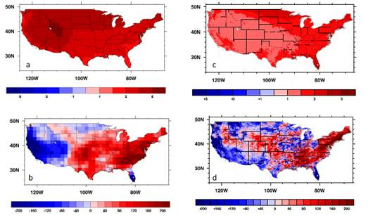
Figure 4. Original (150 km resolution) and downscaled (4 km resolution) CCSM temperature
(°C) and precipitation (mm/year) differences between the period of 2090 - 2099 and 2001 - 2010.
a) original CCSM temperature; v) CCSM precipitation; c) downscaled temperature; d) downscaled
precipitation

Stream temperature modeling – Climate-related stream temperature (ST) warming is expected to have profound effects on the biodiversity and function of stream ecosystems (Woodward, et al. 2010). Observational studies of STs during recent decades suggest that stream- specific responses to climate change (CC) will be highly variable. Adaptive management strategies will require that we understand which streams will be more vulnerable to CC and why. Our objective was to predict CONUS-wide ST responses to CC by 2100. We also sought to identify the physical stream features most associated with ST vulnerability to CC. To meet these objectives we conducted a CONUS-wide modeling study of historical, recent, and future STs.

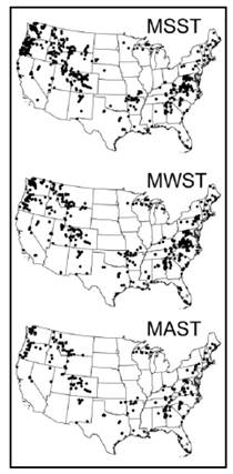
We used ST data from several hundred USGS sites within the CONUS (Fig. 5) to build predictive models of mean summer, mean winter, and mean annual STs based on spatial variation among sites in contemporary (1999-2008) ST and climate conditions. Evaluations showed these models to be both accurate and precise. Analyses revealed that macro-scale patterns of stream biodiversity were most strongly related to summer ST, so this model was used in all subsequent analyses. We assessed how well the model could predict climate-related alterations to ST by comparing responses of modeled and measured changes in historical STs (1972-1998) to variation in historical air temperatures. Modeled STs mimicked observed ST responses to historical climate variation indicating that the ST model could be used to predict thermal responses of streams to future CC.

Figure 5. Distribution of mean summer
(MSST), mean winter (MWST), and mean
annual stream temperature sites (MAST).

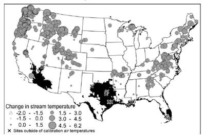
When applied to future climate projections the ST model predicted that STs will warm by 2.2°C on average by 2100. The model predicted greatest ST warming within the Cascade and Appalachian Mountains and least warming in the southeastern USA (Fig. 6). A sensitivity analysis showed that larger changes in ST (ΔST) were associated with warmer future air temperatures, greater air temperature changes, and larger watershed areas. Smaller ΔSTs were associated with streams with greater groundwater influences or that were already relatively warm. Our results suggest that streams will warm considerably by 2100. The ST modeling provided important insight into patterns of ST vulnerability to CC and should help develop testable hypotheses about which adaptation and management strategies are likely to mitigate the effects of CC on STs. This study also provided the basis for predicting the potential thermal- related effects of CC on stream biodiversity by the end of the century.

Figure 6. Spacial variability in MSST vulnerability to CC. Black regions
and Xs represent zones outside of the experience of the ST model.

Hydrologic regime modeling – Streamflow is expected to change with climate change, but a general understanding of how flows will respond is lacking. We sought to advance this understanding by (1) characterizing CONUS-wide spatial variation in flow attributes, (2) modeling how flow attributes vary with current climate and watershed features, and (3) linking these models to downscaled climate projections to predict how flow attributes should change with projected long-term changes in precipitation and air temperature. To characterize flow regimes, we used long-term, daily flow measurements from 601 gauged streams whose watersheds were in relatively unimpaired, reference condition. We characterized flow in terms of both a multivariable classification of sites derived from several individual flow attributes and the continuous variation in individual aspects of the flow regime.

Over 200 streamflow variables have been used in the literature to characterize attributes of streamflow potentially relevant to stream ecology. These variables are commonly grouped into five broad categories: magnitude, timing, rate of change, duration, and frequency. Many of the streamflow variables listed in the literature overlap and are partially or largely redundant. In this project we used an iterative process to identify a set of 16 streamflow variables that, in our judgment, could characterize those general aspects of streamflow regimes relevant to stream ecosystem structure and function. We explicitly included a number of variables that quantify streamflow magnitude because stream size is strongly associated with many aspects of stream ecosystem structure and function.

Based on a principal components analysis we identified 5 separate aspects of temporal variation in flow that were uncorrelated among the 601 gauges. The first component represented variation in low-flow (L) conditions. Streams with small values of L tend to be intermittent, whereas high values of L are characteristic of perennial streams. The second component characterized variation in stream size as measured by discharge magnitude (Q). Large values of Q indicate larger discharge. The third component characterized variation in flashiness (F) of flows. High values of F indicate high variability in daily flows with many individual flood events, whereas sites with low values of F have less variable daily flows and fewer, but longer flood events. The fourth component described annual timing (T) of discharge, i.e., when, within a water year, does most of the flow occur. High values describe streams in which cumulative and peak discharge occurs later in the water year compared with streams with low values of T. The last component represented variation among sites in how constant (C) flows were. The high loadings of both the constancy and predictability attributes indicate the variation in predictability of flows was largely associated with constancy of flows rather than predictable seasonal variation in flows (i.e., contingency). High values of this component indicate a more constant and predictable flow throughout the year, whereas lower values of C indicate that variation in flow occurs unpredictably throughout the year. Note that high constancy can occur when streams have either consistently low or high flows.

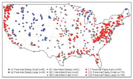
We modeled how both streamflow regimes and individual flow variables responded to projected climate change. We used hierarchical cluster analyses to assign sites into 3 and 8 hydrologic regime classes based on how similar they were to one another in the five aspects of flow. This analysis showed that different classes were broadly associated with different geographic regions, but distinct geographic separation of the classes did not exist. (Fig. 7). We next developed Random Forest models to predict how both streamflow regime class and individual flow variables should vary with climate change. This streamflow regime model used 7 watershed and climate predictor variables: total snow (total precipitation in months with mean temperature < 0°C), precipitation range, scaled June precipitation (scaled precipitation is the fraction of annual precipitation that occurs in the given month), scaled October precipitation, watershed area, mean elevation, and soil permeability. The model had an overall prediction error of 25%, but class-specific errors ranged from 17-34% (Table 1). Intermittent stream classes (noteably B1 and B21) were the most difficult to predict.

Figure 7. Geographic variation in the distribution of streams assigned to
different stream flow regime classes.

Our ability to predict individual flow characteristics varied widely (R2 = 38-91%). The least predictable flow attributes were the number of zero flow events and mean day of year at which peak flow occurred. The most predictable characteristic was mean day of year at which 50% of cumulative annual flow occurred. The most frequently used predictors were relative dryness – the ratio of potential evapotransporation to mean annual precipitation (10 times), long-term mean maximum annual air temperature, long-term total annual precipitation within the watershed, long-term mean annual minimum precipitation within the watershed, mean soil permeability within the watershed, and watershed area.


	A1	A2	B1	B21	B22	C1	C21	C22	Class Error
A1	54		2			1	7	1	17%
A2	4	28						6	26%
B1	3		36	3	8	4	5	3	42%
B21			1	24	3	1	11	2	43%
B22			1	1	33		2	6	23%
C1			6	1		54	3	5	22%
C21			5	4	1	2	151	13	14%
C22	4	3	5	2	3	5	14	70	34%

Table 1. Classification matrix showing class-specific predition errors by the Random Forest
model. The shaded diagonal cells show correct predictions.

We then used the downscaled climate projections to predict how climate change would affect flow regime class and individual flow variables by 2100. Overall, 14% (83 of 601) of streams were predicted to change major class by 2100 (Table 2). 29% (172 of 601) of streams were predicted to change either major or minor class between 2000 and 2100. These projections suggest that the intermittent stream classes will undergo the greatest changes with several of them moving into the perennial flashy classes - 36% (51 of 141). In contrast, many small flashy perennial streams are also projected to become intermittent.


	A1	A2	B1	B21	B22	C1	C21	C22	Class Error
A1	54		2			1	7	1	17%
A2	4	28						6	26%
B1	3		36	3	8	4	5	3	42%
B21			1	24	3	1	11	2	43%
B22			1	1	33		2	6	23%
C1			6	1		54	3	5	22%
C21			5	4	1	2	151	13	14%
C22	4	3	5	2	3	5	14	70	34%

Table 2. Classification matrix showing class-specific predition errors by the Random Forest
model. The shade ddiagonal cells show correct predictions

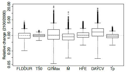
Seven flow variables that were associated with invertebrate biodiversity exhibited variable responses to projected climate change (Fig. 8). On average, the coefficient of variation of daily flows was predicted to generally increase with climate change, and seasonality in flows (contingency) was predicted to decrease. Other flow variables showed less directional changes, and among site variability of these factors did not change.

Figure 8. Relative change in 7 flow variables related to invertebrate biodiversity
(FLDDUR - flood duration, T50 = day of water year at which 50% of cumulative
flow occurs, Q7Max = mean 7 day maximum flow, M = contingency, HFE = number
of high-flow events, DAYCV = foefficient of variation in mean daily discharge,
Tp = day of water year at which peak flow occurs).

Biodiversity modeling – Species distribution models (SDMs) have been increasingly used to model how habitat suitability (and hence the likelihood that a taxon will occur at a site) should vary over space and time in terms of the environmental factors used in the model. Site suitability is scaled from 0 to 1 with 0 implying conditions that cannot support a viable population of a species and 1 implying ideal conditions. These models can be used to examine how both individual taxon probabilities of occurrence and site biodiversity (species composition) vary with climate and other factors. We developed 4 predictive models for stream invertebrate biodiversity with data from 1313 reference-quality sites that were sampled in support of the EPA’s 2008-2009 National Rivers and Streams Assessment (NRSA). These models included a western mountainous/xeric region model, a plains and lowland model, an eastern highlands model, and a model that covered the entire CONUS. Calibration of the CONUS-wide model resulted in the selection of 5 climate sensitive variables that best predicted spatial variation in species distributions: mean summer stream temperature, flow contingency (seasonality), day at which 50 percent of flow is reached, number of high flow events, and 7 day maximum discharge. Model performance as measured by the agreement between observed (O) and predicted (E) taxa richness (O/E) was similar to many previously developed models.

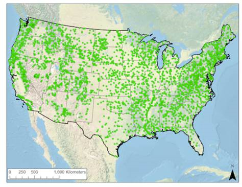
Importantly, model predictions were sufficiently accurate and precise to allow assessment of ecologically meaningful changes in biodiversity at both individual sites and the CONUS as a whole. We applied these models to the 3,806 sites that were used in the NRSA assessment (Fig. 9).

Figure 9. Locations of 3,806 NRSA sites used to project how invertebrate
biodiversity is likely to respond climate change.

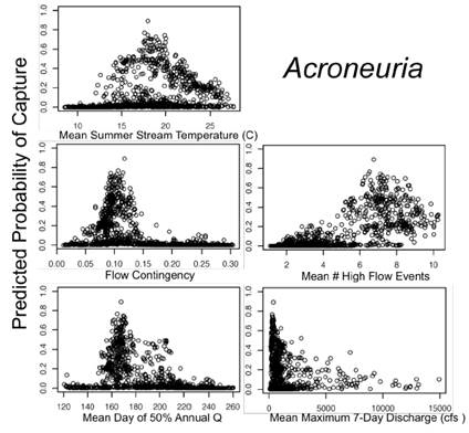
These sites included reference and non-reference quality streams. The model made predictions that were ecologically sensible in terms of how individual taxa are generally distributed across environmental gradients (e.g., Fig. 10). When site-specific predictions of probabilities of occurrence were aggregated to estimate local taxa richness, the model predicted that taxa richness should generally decline with mean summer stream temperature, day at which 50% of annual flow was reached, and mean maximum 7-day discharge and generally increase with flow contingency (seasonal predictability) and the number of high flow events.

Figure 10. Example of how predicted probabilities of capture of an individual
tax (the stonefly Acroneuria) vary across the 3,806 NRSA sites in relation to
5 climate-sensitive environmental variables.

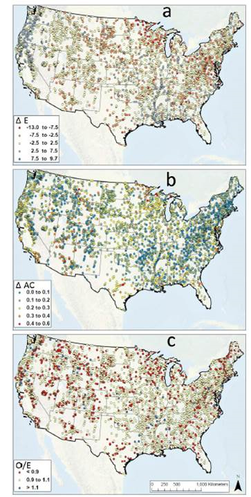
To examine the potential effect of predicted climate change on biodiversity, we compared SDM predictions for 2000-2010 with those for 2090-2100. Site-specific responses to climate change varied markedly in magnitude but showed little geographic coherence. For example, local taxonomic richness was predicted to decrease by as much as 13 taxa and increase by almost 10 taxa (Fig. 11a). Many, although not all, streams in the Pacific Northwest were predicted to increase in richness, whereas in other parts of the CONUS predicted changes in richness were generally negative. However, sites that were in close proximity to one another were often predicted to increase, decrease, or not change in richness. A sensitivity analysis showed that the sites at which richness was most likely to be affected by climate change had MSST of ~ 21°C with decreasing sensitivity at lower and higher MSST. Predicted changes between 2000 and 2100 in taxa composition (as measured by the Bray-Curtis dissimilarity index) were similarly variable and few obvious regional patterns were evident (Fig. 11b). When the predicted site-specific changes in individual taxon probabilities of occurrence were aggregated across all 3,806 sites within the CONUS, 287 taxa were predicted to increase in frequency of occurrence and 252 taxa were predicted to decrease in frequency of occurrence. No CONUS-wide extinctions were predicted, and mean beta diversity (the overall variability in taxa composition among sites) was not predicted to change. Note though that SDMs assume species have no dispersal constraints, so taxa with large predicted changes in range could become extinct under realistic dispersal scenarios.

From a bioassessment context, our analyses indicate that climate induced changes in local biodiversity could significantly compromise the applicability of currently used biological indices. These indices are based on measures of departure between observed taxa and those expected to occur under reference conditions. Most bioassessment programs in the USA base assessments of individual site condition on estimates of reference conditions derived from data collected between 1980 and 2010. By 2100, climate induced changes in biotic composition would result in many reference sites being assessed as biologically impaired (Fig. 11c) relative to currently estimated reference conditions. Indices based on 1980-2010 reference conditions could still be applied later in the 21st century, but regulatory agencies would likely need to tease out climate effects from the effects of those pollutants and water body alterations that fall within the jurisdiction of the Clean Water Act. These adjustments would need to be done on a site-specific basis given the expected variable response of local faunas to climate change (Fig. 11). The alternative is to accept shifting climate-induced baselines when assessing whether water bodies are meeting their aquatic life use designations.

Figure 11. Geographic variation in (a) predicted climate-induced
changes in invertebrate taxonomic riches (E), (b) assemblage
composition (AC) and (c) O/E index values. Predictions are
for 2100.

Conclusions:

Our results indicate that projected climate change by the end of the century (2100) is expected to have substantial effects on the thermal and hydrologic regimes of stream ecosystems and that these thermal and hydrologic changes will affect both local (site) and regional biodiversity. Effects will not be uniform across the CONUS though, and some sites and regions will be much more vulnerable to climate change than other sites and regions. The magnitude and variability of changes in biodiversity will substantially affect the interpretation of currently used indices of biological condition.

Journal Articles on this Report : 11 Displayed | Download in RIS Format

Publications Views
Other project views:	All 73 publications	14 publications in selected types	All 12 journal articles

Publications
Type	Citation	Project	Document Sources
Journal Article	Deng B, Liu S, Xiao W, Wang W, Jin J, Lee X. Evaluation of the CLM4 Lake Model at a large and shallow freshwater lake. Journal of Hydrometeorology 2013;14(2):636-649.	R834186 (2012) R834186 (Final)	Full-text: Yale University-Full Text PDF Exit Abstract: AMS Journals-Abstract Exit Other: AMS Journals-Full Text PDF Exit
Journal Article	Gu H, Jin J, Wu Y, Ek MB, Subin ZM. Calibration and validation of lake surface temperature simulations with the coupled WRF-lake model. Climatic Change 2015;129(3-4):471-483.	R834186 (Final)	Full-text: Research Gate-Abstract & Full Text PDF Exit Abstract: SpringerLink-Abstract Exit
Journal Article	Hill RA, Hawkins CP, Carlisle DM. Predicting thermal reference conditions for USA streams and rivers. Freshwater Science 2013;32(1):39-55.	R834186 (2011) R834186 (2012) R834186 (Final)	Full-text: BioOne-Full Text HTML Exit Abstract: BioOne-Abstract Exit Other: BioOne-Full Text PDF Exit
Journal Article	Hill RA, Hawkins CP, Jin J. Predicting thermal vulnerability of stream and river ecosystems to climate change. Climatic Change 2014;125(3-4):399-412.	R834186 (Final)	Abstract: Springer-Abstract Exit
Journal Article	Hill RA, Hawkins CP. Using modelled stream temperatures to predict macro-spatial patterns of stream invertebrate biodiversity. Freshwater Biology 2014;59(12):2632-2644.	R834186 (Final)	Full-text: Wiley-Full Text PDF Exit Abstract: Wiley-Abstract Exit
Journal Article	Jin J, Miller NL. Improvement of snowpack simulations in a regional climate model. Hydrological Processes 2011;25(14):2202-2210.	R834186 (2010) R834186 (2011) R834186 (2012) R834186 (Final)	Full-text: University of California-Full Text PDF Exit Abstract: Wiley-Abstract Exit
Journal Article	Jin J, Miller NL. Regional simulations to quantify land use change and irrigation impacts on hydroclimate in the California Central Valley. Theoretical and Applied Climatology 2011;104(3-4):429-442.	R834186 (2010) R834186 (2011) R834186 (2012) R834186 (Final)	Full-text: Sringer-Full Text PDF Exit Abstract: Springer-Abstract Exit Other: ResearchGate-Full Text PDF Exit
Journal Article	Jin J, Wen L. Evaluation of snowmelt simulation in the Weather Research and Forecasting model. Journal of Geophysical Research-Atmospheres 2012;117(D10):D10110 (16 pp.).	R834186 (2011) R834186 (2012) R834186 (Final)	Full-text: Wiley-Full Text HTML Exit Abstract: Wiley Online-Abstract Exit Other: Wiley-Full Text PDF Exit
Journal Article	Li L, Li W, Jin J. Improvements in WRF simulation skills of southeastern United States summer rainfall:physical parameterization and horizontal resolution. Climate Dynamics 2014;43(7-8):2077-2091.	R834186 (Final)	Abstract: SpringerLink-Abstract Exit
Journal Article	Liao X, Liu Z, Wang Y, Jin J. Spatiotemporal variation in the microclimatic edge effect between wetland and farmland. Journal of Geophysical Research-Atmospheres 2013;118(14):7640-7650.	R834186 (Final)	Full-text: Wiley Online-Full Text HTML Exit Abstract: Wiley Online-Abstract Exit Other: Wiley Online-Full Text PDF Exit
Journal Article	Zhao L, Jin J, Wang S-Y, Ek MB. Integration of remote-sensing data with WRF to improve lake-effect precipitation simulations over the Great Lakes region. Journal of Geophysical Research-Atmospheres 2012;117(D9):D09102 (12 pp.).	R834186 (2011) R834186 (2012) R834186 (Final)	Full-text: Wiley-Full Text HTML Exit Abstract: Wiley-Abstract Exit Other: Wiley-Full Text PDF Exit

Supplemental Keywords:

EPA Regions 1-10, thermal modification, hydrologic modification, modeling, biological indicators, biological assessment, biological integrity, air, RFA, climate change, air pollution effects, atmosphere, RFA, Air, Atmosphere, Air Pollution Effects, climate change

Progress and Final Reports:

Original Abstract

The perspectives, information and conclusions conveyed in research project abstracts, progress reports, final reports, journal abstracts and journal publications convey the viewpoints of the principal investigator and may not represent the views and policies of ORD and EPA. Conclusions drawn by the principal investigators have not been reviewed by the Agency.