Grantee Research Project Results

2010 Progress Report: Integrated Design, Modeling, and Monitoring of Geologic Sequestration of Anthropogenic Carbon Dioxide to Safeguard Sources of Drinking Water

EPA Grant Number: R834386
Title: Integrated Design, Modeling, and Monitoring of Geologic Sequestration of Anthropogenic Carbon Dioxide to Safeguard Sources of Drinking Water
Investigators: McPherson, Brian J. , Solomon, Douglas Kip , Deo, Milind D. , Goel, Ramesh
Current Investigators: McPherson, Brian J. , Deo, Milind D. , Solomon, Douglas Kip , Goel, Ramesh
Institution: University of Utah
EPA Project Officer: Aja, Hayley
Project Period: December 1, 2009 through November 30, 2012 (Extended to November 30, 2013)
Project Period Covered by this Report: March 16, 2010 through March 15,2011
Project Amount: $899,567
RFA: Integrated Design, Modeling, and Monitoring of Geologic Sequestration of Anthropogenic Carbon Dioxide to Safeguard Sources of Drinking Water (2009) RFA Text | Recipients Lists
Research Category: Drinking Water , Water

Objective:

The University of Utah project team will utilize existing CO₂ geologic sequestration (GS) demonstration sites to develop an "Aquifer Risk Assessment Framework," or ARAF. The ARAF will be a systematic framework that researchers may use to assess and quantify potential risks to Underground Sources of Drinking Water (USDWs) at a specific GS site. The most useful application of the ARAF will be determination of optimized engineering conditions that minimize risks to USDWs for a given set of geologic conditions at a specific GS site.

Objectives/Hypothesis: We hypothesize that (1) geologic sequestration will impact USDWs, but (2) at suitable sites, GS will not adversely impact USDWs. The specific objectives of our study are to (1) identify risks specific to USDWs and develop associated Probability Density Functions (PDFs), (2) quantify risks to USDWs by pressure/brine/CO₂ migration through seals, (3) quantify risks to USDWs by lateral migration of pressure/brine/CO₂, and (4) determine conditions that minimize (or eliminate) the risks to USDWs.

Approach: A key to making the ARAF truly effective is to identify which factors (processes, parameters, etc.) are most important with respect to adverse impacts on USDWs, and to achieve this we will use a case-study approach to test and evaluate the specific components with real data and results. The case study sites include (1) the Gordon Creek field in north-central Utah (PRIMARY SITE)--this site has never been subjected to CO₂ injection and will begin injection in 2012; (2) an active CO₂ injection field site in the Permian Basin in western Texas--CO₂ injection at this site began in October 2008 and injection is not slated to cease until 2012 at the earliest; and (3) an active CO₂ injection field site in the San Juan Basin in northern New Mexico--CO₂ injection at this site began in July 2008, and injection ceased in August 2009. The latter two of these field sites are part of the Validation Phase of the Southwest Regional Partnership on Carbon Sequestration, a partnership and project sponsored by the U.S. Department of Energy and its National Energy Technology Laboratory. A PI of this EPA STAR project (Grant No. R834386) also formed the Southwest Regional Partnership and has led that project since 2003. Thus, access to the field sites and associated data are assured. Although the Gordon Creek Field is the primary site for analysis, we plan to include all three of these field sites in the EPA-sponsored Aquifer Risk Assessment Framework (ARAF) STAR project (Grant No. R834386), if at all possible. These three sites represent the three primary permutations of a CCS geologic site, to facilitate evaluation of different stages of risk analysis and framework development. Specifically, Gordon Creek is a new project area slated for future CO₂ injection, and thus it represents a site with no baseline CCS analysis data at the onset of the project. The Permian Basin site represents active CO₂ injection and monitoring with a relatively mature set of fundamental geologic evaluation, monitoring and simulation data to support ARAF development. Finally, San Juan represents a site that has run the full course of CO₂ injection from drilling to well closure (albeit a medium-scale demonstration).

For the ARAF, we will evaluate the properties and attributes that make each of these a capable storage site. We then will quantify selected risks for all three sites, and attempt to quantify all significant risks for one site. We anticipate this approach to provide essential ARAF elements. Additionally, we will examine alternative natural sites that leak CO₂ such as the Crystal Geyser in Utah, to provide context regarding what attributes may compromise storage sites and to evaluate the nature and processes of leakage. We will use simulations to evaluate a range of possible injection scenarios, and use results to evaluate what engineering conditions will minimize risks. Furthermore, we propose a field program in which fundamental geologic, hydrologic, and key environmental tracer data will be used to demonstrate methodology as well as test the concepts derived from our numerical modeling. Finally, we will compare ARAF development at all three sites, especially pre-injection results to post-injection results, to evaluate what aspects of the ARAF are most and least effective.

Progress Summary:

Task 1: Simulation of Natural Analog Sites

Subtask 1.1 Analysis of Known Leakage Sites

Understanding Eruption Mechanisms of CO₂-saturated Cold Geyser: Analogues to Failed CO₂ Sequestration Sites

The purpose of work associated with Subtask 1.1 is to evaluate the processes that may cause or otherwise influence leakage of CO₂ from target reservoirs to USDWs via abandoned wells or other high-permeability conduits. Rather than speculate regarding conceptual models, we started with analysis of a known CO₂ leakage site located in central Utah, just 3 hours drive from the University of Utah. The Crystal Geyser, located near the town of Green River, Utah, emits low levels of CO₂ continuously, and also erupts with a significantly larger emission of CO₂ daily. Whether this system is representative of a failed CCS site is unclear, and thus we made characterization and simulation analysis of this system as a starting point for the ARAF. The following summary of initial analysis of the Crystal Geyser CO₂ leakage site is split into five sections, as a starting point (draft) for submission to a journal.

Introduction

Two basic types of mechanisms could result in CO₂ leakage from geologic sinks (Figure 1). The first mechanism is fast-flow path leakage, which would primarily involve CO₂ movement through either transmissive faults or fractures in the cap rock above the geologic sink [Pruess, 2008] or poorly sealed or failed injection well casings/cement [Bachu and Bennion, 2009; Barlet-Gouedard, et al., 2009] and improperly abandoned wellbores [Gasda, et al., 2004; Nordbotten, et al., 2004; Nordbotten, et al., 2005; Watson and Bachu, 2007]. The second mechanism is slow leakage, which would primarily involve gas transport by diffusion processes [Altevogt and Celia, 2004; Annunziatellis, et al., 2008; Klusman, 2006] and loss of dissolved CO₂ because of hydrodynamic flow of formation water out of the geologic sink [Oldenburg and Lewicki, 2006].

Figure 1. (a) Potential leakage pathway through an abandoned well [Norbotten, et al., 2005]; (b) Changes of geochemical signature above CO₂ injection formation in Weyburn CO₂-enhanced oil recovery site [Emberley, et al., 2004]

Among these addressed risks, one major risk in CO₂ injection sites is a sudden CO₂ eruption from the stored formation. CO₂ is highly compressible fluid, which is enforced to store in the high pressure and temperature formation, typically over the critical condition for CO₂ being supercritical fluid (Pressure: 7.38 MPa and temperature: 31.1°C). If this compressed CO₂ reaches a highly permeable conduit such as a fault that is continuous to the surface, CO₂ leakage could be dramatic. In general, the pressure gradient within these highly permeable conduits radically changes from the stored formation to the surface with atmospheric pressure conditions. In this situation, CO₂ escaped from the stored formation instantaneously reaches the surface while CO₂ experiences adiabatic expansion, which results in Joule-Thomson cooling.

The addressed eruptive mechanisms are analogues to the natural CO₂ eruption mechanisms, which could be found in cold-CO₂ geysers widely spread all around the world (Table 1). Therefore, proper understanding of the eruption mechanisms in cold-CO₂ geysers will aid in predicting conditions favorable to CO₂ eruptions for engineered CO₂ storage sites.

Table 1. CO₂-saturated cold geysers of the world [Glennon and Pfaff, 2005].

Name	Location	Height	Interval	Duration
Crystal Geyser	Green River Utah, USA	1520 meters	1118 hours	1545 minutes
Woodside Geyser (Roadside Geyser)	Woodside Utah, USA	610 meters	28 minutes	1.01.5 hours
Champagne Geyser (Chaffin Ranch Geyser)	Green River Utah, USA	78 meters	2 hours	5 minutes
Ten Mile Geyser	Green River Utah, USA	2.53.5 meters	6 hours 42 minutes	51 seconds
Tumbleweed Geyser	Green River Utah, USA	0.31.5 meters	28.5 minutes	4694 minutes
Unnamed Geyser	Salton Sea California, USA	0.10.5 meters	1060 seconds	Seconds
Jones Fountain of Life	Clearlake California, USA	< 1.0 meters	60 minutes	22 minutes
Cold Water Geyser	Yellowstone Wyoming, USA	0.5 meters	Unknown	10 minutes
Source Intermittente de Vesse	Bellerive, France	16 meters	230270 minutes	4550 minutes
Andernach Geyser	Andernach, Germany	4060 meters	1.54 hours	78 minutes
Boiling Fount Local name: Brubbel	Wallenborn, Germany	23 meters	30 minutes	a few minutes
Mokena Geyser	North Island, New Zealand	0.55 meters	minuteshours	secondsminutes
Povremeni Geyser	Sijarinska, Serbia	20 meters	9 minutes	2 minutes
Herlany Geyser	Herlany, Slovakia	2030 meters	3234 hours	30 minutes
Persi Geyser	Persi, Slovakia	smaller than Herlany Geyser	hours (shorter than Herlany Geyser)	minutes (probably < 30)

Geologic Setting

In the greater Colorado Plateau covering western Utah to southern Colorado shown in Figure 2a, the CO₂ natural reservoirs including Woodside, Farnham, and McElmo Domes are present on the string extending from northwest to southeast [Allis, et al., 2001]. In these reservoirs, CO₂of more than 98% purity is trapped in dome-like structures and has been produced for commercial usages such as dry ice, industrial uses, and CO₂ enhanced oil recovery.

Close to the Green River in the middle of these CO₂ natural reservoir strings, two major faults, the Little Grand Wash and Salt Wash Graben faults, cross from west to east. Several CO₂ saturated natural geysers and springs shown in Table 1 were discovered on top of these two fault lines, and they have been intensively studied in the past [Assayag, et al., 2009; Gouveia and Friedmann, 2006; Heath, et al., 2009; Shipton, et al., 2005]. Among these springs and geysers, we chose one of the CO₂-saturated natural geysers, the Crystal Geyser, to evaluate the cyclic eruption mechanisms of a CO₂-saturated geyser as an analogue to a failed CO₂ sequestration site.

Methodology

To characterize the periodicity and eruption mechanisms of the Crystal Geyser, we collected the time-series changes of pressure and temperature by installing Geokon Model 4500 vibrating-wire piezometers during two different periods--from August 4 to 6 and September 1 to 5. The piezometer uses a pressure-sensitive stainless-steel diaphragm to which a wire is connected; the other end is attached to a fixed position in the body of the instrument. Pressure variations in the fluid deflect the diaphragm, which causes changes in the tension in the wire. The wire is regularly plucked by an electromagnet and the natural frequency of vibration is recorded. This frequency then is interpreted in terms of diaphragm movement and hence pressure change.

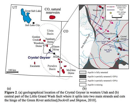
Figure 3. Schematic diagram of well configuration and piezometer installation

During the early trip from August 4 to 6, we first measured the maximum depth where the piezometer could be installed and found that there was an unknown obstacle at the 16 m depth (Figure 3). We were not able to determine the exact reason why the piezometer does not go deeper than 16 m in this study. However, anecdotal reports and discussions with several local people revealed that one individual had used dynamite to enhance the eruption ability of the adjacent geyser and others had tried to use railroad ties to cap the geyser [Shipton et al., 2004; Waltham, 2001]. During our two field-trip periods, we observed a few groups of tourists tossing small rocks into the Crystal Geyser. Interestingly, the researcher who studied the CO₂ exsolution mechanism in the Crystal Geyser 20 years ago [Mayo, et al., 1991] indicated that he had no problem inserting a video camera to a depth greater than 20 meters at that time (Personal Communication with Mayo, 2010).

Due to the presence of an unknown obstacle, one piezometer was installed at the approximate depth of 16 m immediately above the obstacle, and it measured fluid pressure and temperature every 20 seconds. The piezometer was installed at 14:10 pm on August 4, and the observed static pressure and temperature was close to 0.16 MPa and 17.3°C at that time (Figure 4). After the major eruption continued for about 1 hour from 7:30 am to 8:40 am on August 5, however, we noticed that the static pressure and temperature were changed to approximately 0.08 MPa and 17.0°C. We determined that this change occurred because the continuous groundwater discharge through the 0.39 m diameter well was so powerful that the installed piezometer was pushed from a depth of 16 m depth to a depth of 8 m. Therefore, we stopped the monitoring at 12:40 pm immediately after the recharge period and began to record pressure and temperature manually. In the second trip from September 1 to 5, we installed a 1.9 cm-diameter PVC pipe that extended from the top of the well-casing to immediately above the unknown obstacle (Figure 3) and attached two piezometers to the PVC pipe at the depths of 6 m and 13 m, respectively. This configuration was designed to prevent the abrupt movement of the piezometers during the large-scale eruption. The measurements were initiated at 13:10 pm on September 1 at 20 second intervals and they were stopped at 10:30 am on September 5.

Results and Discussion

Field Trip from August 4 to 5

Figure 4 shows the time series changes of pressure and temperature measured at 14:10 pm on August 4 to 12:40 pm on August 5, explicitly conceptualizing the disturbance of fluid pressure and temperature during the eruption period. In detail, our observation using the piezometer installed at a depth of 16 m indicated that both pressure and temperature regularly dropped during the eruption period. In the absence of eruption activity, both the pressure and temperature stayed at consistent levels (0.15 MPa and 17.3°C).

General Characteristics of Eruptions: Intensity and Duration

Two distinctive patterns of eruptions (small and large eruptions) were identified (Figure 4). Twenty-six small-scale eruptions with an average eruption duration of 0.12 hour (7 minutes) occurred during the 16 hours from 15:30 pm on August 4 to 7:30 am on August 5 (Table 2) prior to a single, large-scale eruption, which continued for about an hour. Representative snap-shots of small- and large-scale eruptions are shown in Event B and Event D of Figure 4, respectively.

Table 2. Description of the eruption and recharge sequences during two field-trip periods

Field Trip	Starting time	Ending time	Eruption type	Duration	Comment
8/4-8/6	8/4 15:30 pm	8/5 7:30 am	A-type	16 hour
	8/5 7:30 am	8/5 8:40 am	B-type	1.2 hour
	8/5 8:40 am	8/5 12:40 pm	Recharge	4 hour	Because the levels of static pressure and temperature were changed, we stopped the recording at the piezometer.
	8/5 12:40 pm	8/5 18:15 pm	C-type	5.6 hour	We began to record manually.
	8/5 18:15 pm	8/6 over 1:00 am (?)	Probably D-type	Over 6.8 hour (?)	Eruptions continued past 1:00 am on 8/6. We do not know the exact time when it stopped.
	8/6 over 1:00 am (?)	8/6 10:00 am	Recharge		At 10:00 am on August 6, the geyser was completely drained as shown in Event D of Figure 4.
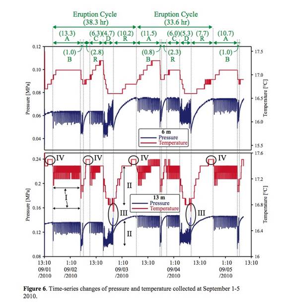
9/1-9/5	9/1 16:50 pm	9/2 6:10 am	A-type	13.3 hour
	9/2 6:10 am	9/2 7:10 am	B-type	1 hour
	9/2 7:10 am	9/2 10:00 am	Recharge	2.8 hour
	9/2 10:00 am	9/2 16:20 pm	C-type	6.3 hour
	9/2 16:20 pm	9/2 21:00 pm	D-type	4.7 hour	PVC pipe attached to piezometers is broken. The level of static pressure and temperature was changed slightly.
	9/2 21:00 pm	9/3 7:10 am	Recharge	10.2 hour
	9/3 7:10 am	9/3 18:40 pm	A-type	11.5 hour
	9/3 18:40 pm	9/3 19:30 pm	B-type	0.8 hour
	9/3 19:30 pm	9/3 21:50 pm	Recharge	2.3 hour
	9/3 21:50 pm	9/4 3:50 am	C-type	6 hour
	9/4 3:50 am	9/4 9:10 am	D-type	5.3 hour
	9/4 9:10 am	9/4 19:50 pm	Recharge	7.7 hour
	9/4 19:50 pm	9/5 6:30 am	A-type	10.7 hour
	9/5 6:30 am	9/5 7:30 am	B-type	1 hour

Multiple Small-Scale Eruptions: In general, during the 5 to 10 minutes prior to every small-scale eruption, we observed that CO₂ bubbles were actively emitted within the geyser (Event A in Figure 4), indicating that CO₂-saturated brine reached the boiling point and started to exsolve CO₂gas from CO₂-dissolved brine. Despite the notable change inside the well, the water pool around the geyser stayed calm during this period. Five to 10 minutes later, the notable small-scale eruption began through the hole at the contact between the well and travertine surface. Because the intensity of the geyser eruption was still small, water discharge did not reach the top of the well casing but flew through the hole at the contact between the well and travertine surface. Soon, the water discharge reached the well casing top (Event B of Figure 4) and the eruption continued approximately 0.12 hour (7 minutes). When the small-scale eruption activity stopped, the water did not bubble anymore but a notable amount of CO₂ gas was emitted instantaneously at the casing top with hissing sounds (Event C of Figure 4). Interestingly, our field observation addressing the sequence of CO₂-driven cold geyser eruption was similar to the field observation and numerical experiments of temperature-driven hot geyser [Ingebritsen and Rojstaczer, 1993 and 1996; White, 1967]. In the hot geyser, there was a period of liquid-only discharge at the beginning of the eruption, and the condition changed to two-phase flow, indicating both water and steam were emitted together. At the final stage, the water discharge stopped early and then only steam was emitted.

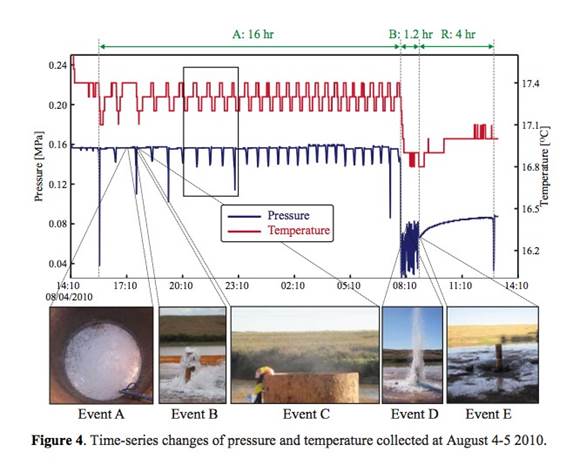
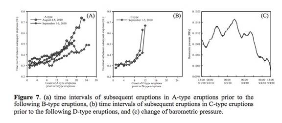
Single Large-Scale Eruption: Single large-scale eruption, characterized by large reduction of both pressure and temperature and, at the same time, longer eruption duration, occurred from 7:30 am to 8:40 am on August 5 after a series of multiple small- scale eruptions (Figure 4). In detail, we differentiated between large- and small-scale eruptions based on three major components such as intensity, duration, and drainage period. First, the intensity of the large-scale eruption was strong and, due to the power of instantaneous CO₂ gas emission, the water column reached approximately over 10 m above the surface (Event D in Figure 4) but it only reached the casing top in the small-scale eruption (Event B in Figure 4). Due to the intensity difference, both the pressure and temperature drop was significantly larger in the large-scale eruption than in the small-scale eruption. Second, the average duration of the small-scale eruptions was approximately 0.12 hour (7.2 minutes) but that of large-scale eruption was 1.2 hours. Finally, we did not observe any change of height in the water pool around the geyser immediately after the small-scale eruption although a slight decrease of hydrostatic pressure was measured. However, after the large-scale eruption of 1.2 hours ceased, the water pool was completely drained into the geyser (Event E in Figure 4), and the water level inside the geyser well was approximately 2.5 to 3 m below the surface.

After the end of the intensive large-scale eruption, the recharge period began from 8:40 am and ended at 12:40 pm on August 5 with the first occurrence of a small-scale eruption. As we addressed in the Methodology section, at this moment, we discovered that the static levels of pressure and temperature had changed. Therefore, we stopped the piezometer measurement and recorded manually until 10:00 am on August 6. After the recharge period ended at 12:40 pm on August 5, we observed that an addition series of multiple small-scale eruptions continued (Table 2). The general characteristics of the small-scale eruptions were similar to those observed on August 4, but on August 5, the duration of the multiple small-scale eruptions prior to the single large-scale eruption was only 5.6 hours, which was approximately three times shorter than those the previous day (16 hours). After the multiple small-scale eruptions, the single large-scale eruption began at 18:15 pm on August 5 and continued past 1:00 am on August 6. Although we did not observe the exact time when this large eruption ended, its duration was more than 6.8 hours. The well was completely dry when we visited it at 7:00 am on the morning of August 6.

Identification of Single- and Large-Scale Eruptions: From the observation of August 4 field trip, we identified four different eruption patterns (A, B, C, and D) and two recharge periods in the Crystal Geyser (Table 2). A-type is characterized as multiple small-scale eruptions that continued for 16 hours. Immediately after the end of the A-type eruption period, the B-type eruption, which is characterized by a single large-scale eruption, continued for 1.2 hours. At the end of the B-type eruption, the level of groundwater inside the well fell to 2-3 m under the surface. A recharge period of approximately 4 hours was required prior to the occurrence of additional multiple small- scale eruptions, which we identified as the C-type eruption. The C-type eruption was multiple small-scale eruptions similar to A-type eruptions but the duration of the C-type eruption was shorter (5.6 hours). After the C-type eruption ended, the D-type eruption--a single large-scale eruption--continued for more than 6.8 hours. The identified patterns were captured in detail during the second field trip on September 1 to 5, and will be discussed further in the paper entitled "Coupled Natures of CO₂-Driven Geyser Activity: Based on the Observation of Multiple Small-Scale Eruptions." We determined that all eruptions had three regular phases: pre-eruption, eruption, and recharge (Figure 5). In addition, the changes in pressure and temperature during the eruption period were closely intercorrelated, similar to the observation of the other CO₂-driven cold geyser in New Zealand [Lu, et al., 2005].

During the pre-eruption period, pressure was consistent but a 0.1°C increase in temperature was observed (Figure 5). We believe that this slight temperature increase was due to the increase of kinetic energy caused by CO₂ bubbling in the system and the recharge of relatively hot groundwater from deeper formations. Prior to the pre-eruption period, CO₂ bubbling, as shown in Event A of Figure 4, has not been observed within the geyser, which implies that the slight increase of temperature is somehow related to CO₂ bubbling.

During the eruption period, we observed that both pressure and temperature dropped instantaneously (Figure 5). The reduction of hydrostatic pressure indicates that a certain portion of the water column above the piezometer is displaced with CO₂ bubbles. The instantaneous temperature drop is primarily caused by the cooling contribution from the Joule-Thomson effect and endothermic CO₂ exsolution. The Joule-Thomson effect addressed the temperature drop of CO₂ due to the instantaneous expansion of CO₂ gas volume induced by the pressure reduction during the isenthalpic condition (enthalpy change is zero). This has been studied previously [Han, et al., 2010; Katz and Lee, 1990; Oldenburg, 2007]. In the Crystal Geyser, CO₂ gas is exsolved from CO₂-saturated brine at a certain depth below the surface. Immediately after the nucleation of the CO₂ gas bubble, the CO₂ gas will migrate vertically through the water column of the well because of its buoyancy. As CO₂ gas migrates closer to the surface, the hydrostatic pressure falls and the volume of CO₂ gas increases. If these processes occur simultaneously, we could expect a substantial decrease in temperature. Further, it is well understood that the CO₂ dissolution process is an exothermic reaction within the appropriate range of enthalpy variations from -440 to -200 kJ/kg at temperatures ranging from 25°C to 100°C [Carroll, et al., 1991; Duan and Sun, 2003; Ellis, 1959; Ellis and Golding, 1963; Koschel, et al., 2006]. Because the reaction is an exothermic reaction, heat evolves as the CO₂ dissolves in the brine. The CO₂ exsolution from liquid is simply the opposite process of the CO₂ dissolution in liquid. In principle, the corresponding enthalpy change in CO₂ exsolution is going to be the same with CO₂ dissolution except it is defined as an endothermic reaction; the brine cools as the CO₂ gas exsolves from the fluid. Therefore, we attribute the slight temperature decrease observed during the eruption period to the cooling contribution from both the Joule-Thomson effect and CO₂ exsolution. Interestingly, we found that the temperature decreased again after the recharge phase. We believe this occurs because the temperature change in the system is relatively slow compared to the pressure change.

Field Trip from September 1 to 5

General Characteristic of Eruptions: Intensity and Duration: The observation from the second field trip on September 1 to 5 revealed the consistent eruption cycle observed during the first field trip. Thus, we were able to construct a clearer eruption cycle for the Crystal Geyser (Figure 6). As we discussed in the previous section, Identification of Single- and Large-Scale Eruptions, the data from the September field trip also confirmed that the eruption cycle is composed of four different eruption types (A-, B-, C-, and D-types) and two recharge periods (Table 2 and Figure 6). Two eruption cycles were captured and the time scales for these two cycles were 38.3 hours and 33.6 hours, respectively.

Within the eruption cycle, both B- and D-type eruptions are characterized as large-scale eruptions, which occurred immediately after the end of A- and C-type eruptions, respectively. Interestingly, there are distinctive features between B- and D-type eruptions, including eruption duration, recharge period, and the characteristic of multiple small-scale eruptions occurring prior to a large-scale eruption.

First, the D-type eruption was always longer than the B-type eruption (Figure 6 and Table 2). Within the first eruption cycle in Figure 6, B- and D-type eruptions continued for 0.8 and 4.7 hours, respectively.

Second, the D-type eruption always required a longer recharge period until the first small-scale eruption occurred.

Finally, prior to these two large-scale eruptions (B- and D-types), multiple small-scale eruptions (A- and C-types) occurred but their number of eruptions differed. As seen in Figure 7, the number of A-type eruptions that occurred was less than the number of C-type eruptions. These characteristics were consistently observed during both the August and September field trips. This finding differs from the general understanding that the periodic eruption of a geyser shows the bimodal pattern [Azzalini and Bowman, 1990; Rinehart, 1980]. However, despite this finding, we were not able to determine the exact reason why two single large-scale eruptions occurred with different eruption durations.

The previous study associated with a temperature-driven hot geyser discovered that the change of barometric pressure could affect eruption cycles [Rinehart, 1972; Rojstaczer, et al., 2003; White, 1967]. In general, although the boiling temperature of pure water at atmospheric conditions is 100°C, it varies with pressure conditions and the amount of dissolved gas content in the water. Specific to the pressure variation, the boiling temperature increases with depth as the hydrostatic pressure increases but it decreases as the atmospheric pressure is reduced. For this reason, the change of barometric pressure could affect the boiling temperature in the hot geyser, resulting in a change of the eruption characteristics of the geyser. For example, previous studies showed that as the barometric pressure decreased, the discharge amount from the geyser is increased and the eruption interval becomes shortened [Rinehart, 1972; White, 1967]. To investigate the effect of barometric pressure change, we gathered barometric pressure data from the closest weather station located at Moab, Utah (Figure 7c). During the 5 days from September 1 to 5, barometric pressure reached a maximum (> 0.016 MPa) the morning of September 3 and decreased continuously until 13:00 (1:00 pm) on September 5.

Although barometric pressure changes were observed, we found that this external force did not control the interval between the multiple small-scale eruptions. We observed that the interval gets smaller as the time for the single large-scale eruption approaches (Figure 7 a and b). This specific trend, which was observed only at the Crystal Geyser, confirmed that the event of the small-scale eruptions induced the reduction of hydrostatic pressure causing the exsolution of more CO₂ gas from the CO₂-saturated brine. Therefore, a series of multiple small-scale eruptions (A- and C-types) could trigger a single large-scale eruption (B- and D-types).

Specific Characteristic (I, II, III, and IV) in Eruption Cycle: We observed four different characteristics (I, II, III, and IV), identified in Figure 6, in the eruption cycles. Both characteristics I and II represent the systematic coupled-nature of pressure and temperature due to CO₂-related chemical reactions such as Joule-Thomson cooling and endothermic CO₂ exsolution. Typically, larger-scale eruptions caused more significant reduction of both pressure and temperature than small-scale eruptions (comparison between I and II). In addition, although temperature change during the large scale-eruption distinctively appeared at both 6 m and 13 m, we found that thermal effect is relatively smaller at the shallower depth. This is because the CO₂ bubbles, which are relatively colder than the surrounding fluid due to Joule-Thomson cooling and endothermic CO₂ exsolution, lose their heat due to thermal conduction while they migrate vertically. For this reason, thermal disturbance caused by multiple small-scale eruptions was distinctive at 16 m but not at 6 m. Characteristic III specifically pointed out the process at the end of large-scale eruptions, where the measured hydrostatic pressure is increased but temperature reached the minimum. At the end of the large-scale eruption continued over 4 hours, the temperature of the fluid in the geyser becomes cool due to the continuous CO₂ exsolution and adiabatic cooling processes. The decrease in temperature induced an increase in brine density, which resulted in an increase of the hydrostatic pressure in the geyser. Finally, we observed the slight increase of temperature immediately before multiple small-scale eruptions (characteristic IV in Figure 6). As we discussed earlier, the slight increase of temperature shown in Figure 5 was considered to be due to the increase of kinetic energy caused by CO₂ bubbling in the system and the recharge of relatively hot groundwater from deeper formations.

Conceptual Description of CO₂-Driven Cold Geyser Eruption Mechanisms

CO₂ exsolution results in the decrease of the hydrostatic pressure and also reduces the temperature during both small and large eruption periods. Based on our observations, we developed a conceptual model describing the physical and chemical mechanisms causing cyclical eruptions from a CO₂-driven cold geyser. Stage A in Figure 8 indicates the start of the geysering cycle, when the water reaches the top of the well and overflows. During the overflow process, CO₂ exsolves from the CO₂-saturated water at the depth above the critical exsolution pressure point and thus, CO₂ bubbles begin to form in the water. At Stage B, the refilling of the well at the bottom by the recharging aquifer, causes the water level to rise in the well. When the overflow starts, the bubbles rising with the fluid begin to decrease the hydrostatic pressure at the top of the well (see the hydrostatic line in Stage B). The water level is fixed at the wellhead, so any slight density change progresses down the well as gaseous CO₂ is released from solution, and the rate of bubble formation increases. CO₂ bubbles continue coalescing and the depth of the critical CO₂ exsolution pressure point becomes deeper as more CO₂ bubbles are exsolved, which results in a further decrease of the hydrostatic pressure. At Stage C, eruption begins once the depth of the critical CO₂ exsolution pressure point reaches the deepest point. At this stage, the hydrostatic pressure reaches its minimum. Once the eruption is over at Stage D, CO₂ bubbles escape to the atmosphere, causing the water leve within the well to decrease. In addition, the depth of CO₂ exsolution pressure becomes shallower. Finally, CO₂-saturated brine is recharged from the bottom of well and Stage A begins again.

Task 2: Simulation of Engineered Storage Sites (San Juan Basin, SACROC, Gordon Creek)

The ARAF team is evaluating multiple site case studies for the sake of analyzing the risks at sites at different stages of CCS operation, including three sites now available for access and analysis. These sites include:

The Gordon Creek field in north-central Utah, just 25 miles from the original Farnham Dome site (and thus our baseline geologic and hydrologic knowledge is very solid). This site has never been subjected to CO₂ injection, and will not begin injection for at least 1 year from now.
Our SWP (Phase 2) field site in the Permian Basin in western Texas; we started CO₂ injection at this site in October 2008, and injection is not slated to cease until 2010 at the earliest.
Our SWP (Phase 2) field site in the San Juan Basin in northern New Mexico; we started CO₂ injection at this site in July 2008, and injection is ceasing this week (the week of August 17, 2009).

We plan to include all three of these field sites in the ARAF STAR project to some extent, but our priority is the Gordon Creek field, and thus it will receive most of our time and effort. These three sites represent the three primary permutations of a CCS geologic site, to facilitate evaluation of different stages of risk analysis and framework development. Specifically, Gordon Creek is a new project area slated for future CO₂ injection, and thus it represents a site with no baseline CCS analysis or data at the onset of the project. The Permian Basin site represents active CO₂ injection and monitoring with a relatively mature fundamental geologic evaluation, and substantial monitoring and simulation data to support ARAF development. Finally, San Juan represents a site that has run the full course of CO₂ injection from drilling to well closure (albeit a medium-scale demonstration).

The primary focus for the first year of the ARAF project was the Gordon Creek field, representing a site in pre-injection mode.

Task 2.1: Analysis of Pre-Injection Site: Gordon Creek Field, Utah

Geologic Model Development and Analysis

The Gordon Creek project area is one of the three field sites proposed in the EPA-sponsored ARAF STAR project we are performing. Gordon Creek field is a proposed large-scale CO₂ injection site of the Southwest Regional Partnership on Carbon Sequestration (SWP). Gordon Creek field is a natural gas field located in T14S, R7-8E, Carbon County, Utah, producing methane from the Cretaceous Ferron Sandstone (Figure 1). The Permian White Rim Sandstone provides an estimated rate of 8,900 MCFPD of 98.82% CO₂ (Morgan and Chidsey, 1991).

Gordon Creek field is located on the eastern flank of Wasatch Plateau. Closed anticline structure trending north-south in the field is approximately 9 miles long and 5 miles wide and serves as a structural trap for methane gas in the Ferron Sandstone and possibly CO₂ in the White Rim. Geology in the proposed site exhibits a stacked system of alternating reservoirs and seals, which provides optimal conditions for geologic CO₂ storage. The target CO₂ injection formations are the Jurassic Navajo and Entrada formations due to their intermediate depth and the current use of salt water disposal into the Navajo.

Figure 9. Location map of Gordon Creek project area, Carbon County, Utah.

In this task, we focused on developing a site-specific static model based on the data collected specific to the Gordon Creek site. The location of the Gordon Creek site is illustrated in Figure 9. We gathered the stratigraphic formation top picks, well information, and well log images available from the project site. The distribution of wells in the site is shown in Figure 10. The well log images were digitized into the digital format (LAS).

Figure 10. Location of wells with digitized gamma ray logs. Vertical exaggeration is 2x.

For the static geologic model development, we utilized the formation tops data tied to isochore surfaces. The resulting static model within the model boundary is shown in Figure 11. The model domain covers 8.2 km by 9.2 km in the x and y direction, centered at the proposed injection well. The constructed model contains 13 formations starting with the Cretaceous Mancos shale on top to the Kaibab formation at the bottom.

Figure 12 illustrates the grid setting of our target formations, Navajo and Entrada formations. Currently, the grid configuration is 41 x 46 x 65 cells in the x, y, and z direction, respectively, with a cell dimension of 200 m by 200 m. Five cells were equally spaced vertically in each formation. The average thickness of target formations within the model domain is found to be approximately 19.2 m and 63 m, respectively, for the Navajo and Entrada formations.

Figure 11. Stratigraphic distribution of geologic formations within the Gordon Creek site model boundary. Vertical exaggeration is 2x.

Figure 12. Grid settings of target formations (Navajo and Entrada). Horizontal cell dimension is 200 m x 200m. Vertical exaggeration is 2x.

Overpressure Sensitivity Study

Using the initial Gordon Creek 3-D grid, we evaluated conditions under which overpressures might form in the Navajo Sandstone, the primary storage target reservoir. Because we have very little data (e.g., permeability, porosity, etc.) for the area to date, this initial analysis is a sensitivity study by definition.

For this area, the fracture gradient approaches 80% of lithostatic pressure, and thus these simulations provide an initial glimpse regarding conditions that will lead to seal failure via fractures. This initial analysis will serve as a starting point for development of probability density functions for this pre-injection site. Figure 13 suggests that for the specific thickness and geometry of the preliminary model, overpressures may develop only if permeabilities are less than approximately 5 x 10^-17 m², for any significant CO₂ injection rates (greater than 1000 tons per year, for example).

Likewise, once CO₂ is injected in the reservoir, the viscosity of the water/brine/CO₂ mixture changes as composition changes. While the viscosity of pure (liquid) CO₂ at storage-reservoir conditions will not exceed 0.1 cP, water/brine viscosities can approach 1 cP, or even higher if oil is in place. Figure 14 indicates that fluid mixtures must approach relatively high viscosities (> approximately 1.5 to 2 cP) to favor overpressure development. These general results are corroborated by re-plotting the results of normalized overpressure as a function of viscosity and permeability (Figure 15).

We will use these general results to limit the parameter space required for development of probability density functions for induced seismicity. We will begin analysis of risk of induced seismicity for the Gordon Creek site during this next quarter.

Figure 13. Isometric projection of normalized overpressure versus injection rate and permeability, calculated for the generalized 3-D Gordon Creek site grid.

Figure 14. Isometric projection of normalized overpressure versus injection rate and fluid (injected) viscosity, calculated for the generalized 3-D Gordon Creek site grid.

Figure 15. Isometric projection of normalized overpressure versus permeability and fluid (injected) viscosity, calculated for the generalized 3-D Gordon Creek site grid.

Task 3: Identification of Risk Elements and Development of PDFs

Subtask 3.2: Methods of Probability Density Function (PDF) Development

Analysis of CO₂ Leakage into Overlying Formations

Given the presence of a major fault located 500 meters from the planned injection site, we will develop probability density functions (PDFs) for risk of (a) leakage through this fault, and (b) induced slip on this fault, following CO₂ injection; we will deliver these PDFs and a detailed description of the process and algorithms used to develop these PDFs. Thus, the subtask 3.2 activities during this first year consisted of two main components.

Development of a methodology for calculating the probability of leakage of CO₂ into USDWs, especially via known (or unknown) fault pathways;
A study of the impact of the fault structure on possible leakage of CO₂ into overlying formations.

A generalized experimental design approach was developed to generate response surfaces and subsequently PDFs of important outcomes (overpressure, free CO₂ concentration, etc.) as functions of significant input variables (porosity, permeability, anisotropy, etc.). Detailed methodology with results will be discussed in the next report. In this report we provide results of the effect of fault structure on CO₂ leakage and possible consequences to USDWs. More details can be found in Pasala (2010).

Faults and fractures provide one of the primary risk factors for leakage in an engineered system. Injected CO₂ may find its way out of the repository and into USDWs. In this part of the project, faults in various settings were examined to determine their influence on CO₂ flow with reservoir rock and fault-affected rock. Fluid flow simulation results in this study help to constrain how engineered sites might best be designed to reduce the risk of leakage, and to examine the possible consequences of a leaking system.

The Navajo sandstone is a good analog for reservoir simulation and study. Porosity values of the Navajo sandstone can be as large as 20 to 30%. Permeability values measured in the Navajo sandstone typically range from 100 to 1000 millidarcies (md), with values as large as 8000 md [Freethy, et al., 1991]. Average permeability values for Navajo sandstone of 450 to 860 md also have been reported. Joints are features that can either enhance permeability or reduce it.

Joints are extension-induced mode I fractures that exhibit only opening displacement (white features in Figure 16). Deformation bands are planar, light-colored, vein-like features formed of ground and crushed sandstone grains and fine powder (dark features in Figure 16). Both joints and deformation bands are found as single features, or in networks, aligned sub-parallel to fault zones. Joints or deformation bands may be found alone, or together, leading to the possibility of a wide range of deformation-induced permeability variation within and near faults.

Figure 16. Typical arrangements of deformation-induced features in faulted sandstone. Arrows show direction of fault slip. Black features are individual/ amalgamated deformation bands. White features are open fractures.

A sealed case with a high permeability fault and its impact on the CO₂ leakage is investigated. The model volume used in all of the above simulations was 600.5 feet by 420 feet in plan and 280 feet thick. Vertical, impermeable faults are assumed to surround a sandstone aquifer that is sealed by low permeability rocks both above and below the aquifer. A 35 x 60 x 40 (84,000 grid blocks) Cartesian grid was used for all simulations. The 35 grid blocks in the X direction are of lengths 16 x 25, 3 x 15, 7.5, 5.0, 3.5, 2.25, 1.5, 1.0, 1.5, 2.25, 3.5, 5.0, 7.5, 15, and 4 x 25 feet. The 60 grid blocks in the Y direction are of lengths of 7 feet each. This makes the areal dimension of the field 600.5 x 420 feet. In the vertical (Z) direction, there were 40 layers of 7 feet each. A vertical, north-south trending fault is located 100 feet west of the injection well and fully penetrates the reservoir/aquifer. The fault is 15.5 feet wide. Fault grid blocks with sides as small as 1 foot are included in the model. Such fine grid blocks resolutions are needed to capture the small physical size of fault zone details.

The reservoir is basically divided into three sections, upper reservoir, sealed middle section, and lower reservoir, as shown in Figure 17. The thicknesses of the upper reservoir and middle seal were 70 feet each.

The injection well used a rate constraint of 100 MSCF/day. Injection was uniform and was selected to occur over the entire thickness of 140 feet (of the reservoir) for 500 days, which means the total amount of gas injected is 50,000 MSCF (50 MMSCF). The basic idea was to observe CO₂ flow paths and investigate a long-term CO₂ injection study.

The success of CO₂ sequestration by deep injection depends on the ability of upper and lateral seals to confine the over-pressured fluid. One potentially serious problem associated with injection into underground formations is the possible leakage of injected CO₂ through or along faults into USDWs. Over long time scales, these faults/fractures may serve as short-circuit pathways for ultimate leakage into upper formations. This is of great concern because leakage of CO₂ in large quantities would compromise the integrity of USDWs.

Figure 17. Front view of the reservoir simulator set-up in the reservoir with horizontal seal case.

Permeable fault-related fractures in sandstone can focus CO₂ flow to leakage points where permeable faults breach reservoir-sealing units and enable injected CO₂ to leak into overlying USDW formations. On the other hand, low-permeability faults can restrict access to fault-bounded CO₂ sequestration volumes. The total amount of gas injected for 500 days was 50,000 MSCF (50 MMSCF). The top and the bottom layers have the same reservoir properties.

Depending on whether the fault zone is characterized by the deformation band or the joint, the permeability of the fault zone could vary by as much as six orders of magnitude (Figure 18).

The sealed middle layer has a permeability and porosity of 0.01 md and 7%. The two end member cases for fault permeability structure as discussed earlier were studied, the high-permeability fault containing open fractures and the low permeability fault containing deformation bands.

Figures 19 and 20 show vertical views of dissolved CO₂ distributions for a deformation band and fractured fault case after 100 and 500 days. The injected gas spreads out in the bottom layers and does not escape into the top reservoir due to reservoir seal. A low permeability fault even though it cut across the entire reservoir does not allow any leakage of CO₂ into the overlying formations.

Figure 21 shows the volume of CO₂ sequestered in the three layers. In the fractured fault case, CO₂ has leaked to the top layer as opposed to in the deformation band fault. The fractured fault broke the seal and migrated into the top layer. About 22.75% of the injected CO₂ has leaked into the upper layer in the fractured fault case. On the other hand, in the deformation band fault, 87.3% of the CO₂ resided in the bottom layer. Basically, there is negligible CO₂ migration into the top layer in this case. Hence, the DB fault almost has no leakage into the USDWs compared to the fractured fault.

Figure 18. Variation in equivalent porosity and permeability of a 1 m³ rock block for two different host rocks as low-k deformation bands (DBs: _ = 0.07, k = 500 mD, 1 mm thick) and high-k fractures (Fracs: aperture = 0.1 mm) are added. The upper line is for host k of 500 mD and porosity of 25%. The lower line is for host k of 50 mD and _ = 0.15. DB identifies deformation bands and Frac identifies fractures.

Figure 19. Dissolved CO₂ distribution in a stacked reservoir system after 500 days for a deformation band fault case.

Figure 20. Dissolved CO₂ distribution in a stacked reservoir system after 500 days for a fractured fault case.

Figure 21. Volume of CO₂ sequestered in the top, middle, and bottom layers in a deformation band, and a fractured fault case.

Task 4: Hydrodynamic Analysis of Tracer, Microbiologic, Chemistry and Physical Field Data and Use of These Data to Calibrate Quantitative Risk Assessment

(e.g. probability of USDW contamination based on a certain event or combinations of events)

Task 4.1: Analysis of Noble Gas Data and Hydrodynamic Interpretation

Introduction

The purpose of subtask 4.1 (noble gas portion of the project) is to measure the ⁴He content of minerals obtained from drill core or cuttings, relate this to pore water concentrations of ⁴He via solubility relationships, and then utilize the derived pore-water concentrations to estimate natural rates of fluid flow. We will evaluate our results by comparing them with more traditional estimates of fluid flow (e.g., based on Darcy's Law), along with results from numerical simulations and with other environmental tracers such as stable isotopes of oxygen and hydrogen in water.

Helium is the decay product of naturally occurring uranium and thorium in rocks and sediments. As ⁴He is produced, it is initially retained by mineral phases in the subsurface; however, eventually this helium diffuses into surrounding pore fluids forming the basis for the ⁴He method of groundwater dating [Solomon, 2000]. As such, the concentration of ⁴He in pore fluids depends strongly on the time in which these fluids have been in contact with helium-producing rocks. In low permeability systems, pore water helium concentrations can rise to large levels. In the extreme case in which pore fluids are completely stagnant, the total mass of helium produced over the life of the geologic formation will be similar to the mass of helium residing in pore fluids and minerals. Differences between the mass produced and the mass currently residing in the system are the result of helium transport processes, the most significant of which is groundwater flow. This concept has been successfully applied to near surface groundwater systems where pore fluids could be accessed using multilevel monitoring wells [Sheldon and Solomon, 2003; Hendry, et al., 2005]. However, it is not practical to install multilevel monitoring wells at the depths proposed for carbon sequestration. Instead, the focus of this component of our research will be to develop a method whereby the helium concentration in pore fluids (within subsurface seals) can be estimated using measurements of the helium content of minerals obtained from drill core or cuttings, along with measurements of the apparent helium solubility in these minerals. The development of this method then will allow us to estimate the mass of ⁴He residing in geologic seals. Comparisons of this mass with that produced over the age of the seals, will allow us to assess the magnitude of fluid flow through the seals over long periods of time. This in turn will allow an evaluation of the degree to which seals can contain injected CO₂.

Progress to Date

Our objectives for Year 1 of the project were to develop a methodology for (1) measuring the helium content of quartz and (2) determining a sample specific partition coefficient; and to calculate the in situ concentration of helium in pore waters. The first step in this process was to develop a method for separating appropriately sized quartz grains from bulk caprock samples.

Separation of Quartz from Bulk Rock Samples

We have successfully obtained high-purity quartz separates from shales using the following procedure.

Approximately 50 grams of each core was disaggregated using a shatterbox for 15 seconds. The samples then were repeatedly rinsed in deionized (DI) water, allowed to settle, and decanted to remove clay particles followed by drying at ambient temperatures. Samples then were dry sieved at 850, 150, and 43 µm. The > 850 µm fraction was disaggregated further with a porcelain mortar and pestle before re-sieving. The 43-150 µm fraction (~10 g) then was treated with 10% nitric acid in an ultrasonic bath for 5 minutes to dissolve carbonate minerals. This was followed by rinsing in DI water, settling, and decanting to remove fine particles. The samples then were treated for 23 times as follows: five-minutes with 5% hydrofluoric acid (HF) in an ultrasonic bath and rinsing with DI water, settling, and decanting. The HF selectively dissolves clays minerals with minimal reaction with quartz. The samples then were dried at ~75°C before magnetic separation using a Frantz machine to remove mafic minerals (those rich in magnesium and iron) such as amphiboles and pyroxenes. This step is particularly important as mafic minerals could retain internally produced ⁴He and are not likely to be in solubility equilibrium with pore fluids.

The above procedure generally yielded between 1.0 and 1.5 g of purified sample of ~95% quartz with the remainder being feldspars with trace amounts of clay. Figure 22 expresses a photomicrograph from a petrographic microscope of a typical sample. The field of view is approximately 500 microns (left side to right side) and the mounting media is clove oil with a refractive index of 1.543. The upper image is with the polarizer crossed while the lower image is with plain light with a single polarizing filter. The dark spots on some of the grains (when viewed under plain polarized light) are trace amounts of clay minerals that could be removed with additional treatments in HF; however, they are unlikely to change either the measurement of ⁴He dissolved in the quartz under in situ conditions, or our determination of the helium partition coefficient.

Figure 22. Photomicrographs of quartz separates obtained from cores of shales (caprock). The upper image was taken with the polarizer crossed while the lower image was with plain light with a single polarizing filter. The field of view is approximately 500 microns from the left to the right side.

Measurement of Helium in Quartz

The ⁴He content of quartz separates was measured by heating the samples at 290 ºC in a custom high-vacuum vessel designed specifically for this project (Figure 23). The vessels were constructed by boring a 1/4 OD copper tube to an ID of 0.225. A stainless steel frit with a pore-diameter of 10 microns was installed inside the copper tube, and then sealed using a swaging tool. After the sample was placed inside the vessel, the end was sealed using a cold welding tool. The other end of the copper tube was flared to 37 ºC to make a high-vacuum seal when connected to the helium analytical system.

The samples are evacuated to high vacuum (< 10⁸ torr) for more than 48 hours to remove any residual water and noble gases that are either dissolved in the water or trapped as a gas phase by the residual water. The stainless steel frit is particularly important for this evacuation as it prevents loss of sample and protects the high vacuum system from particulates.

Figure 23. High vacuum container for measuring helium in quartz. The sample is located in the right side of the container. A stainless steel frit with a pore size of 10 microns (shown above the sampler for illustration) has been swaged into the copper tube. The frit retains the sample within the tube especially during initial pumpout. The metal pinch clamp can be opened and closed numerous times and till a high-vacuum seal is achieved. The left end is flared to produce a high-vacuum seal when connected to the helium analytical system. The container allows both the initial measurement of in situ helium in the quartz and the impregnation of tank helium to be made in the same container. Because of the potential for also impregnating the container with trace amounts of helium, the sample is removed after impregnation and placed in a new container before measuring the amount of impregnated helium.

Preliminary Results

One sample has completed the entire measurement cycle with the results shown in Table 3.

Table 3. Results of helium and neon measurements on sample B-1-2698.2

Step	⁴He (ccSTP/g)	²⁰Ne (ccSTP/g)	R/R_a	Comments
Initial heating at 290 ˚C for 4.5 days	1.59 X 10⁷	2.45 X 10⁸	0.108	Total sample mass = 0.5390 g
Additional heating at 290 ˚C for 7 days	1.41 X 10⁸	1.99 X 10⁸	0.148	Result shows that approximately 90% of He was removed during initial heating.
Filled to 3.596 Torr with pure helium, heated to 290 ˚C for 11 days. Placed in new container and heated at 290 ˚C for 12 days.	8.76 X 10⁷	1.36 X 10⁸	0.169	Mass placed in new container = 0.3068 g.

Following the approach of Lehmann, et al. (2003) the partitioning coefficient can be expressed as the helium-accessible volume (V₂) of quartz by applying the ideal gas law as:

V₂= V₁ (p₁/p₂) (T₂/T₁) Eq. 1

where,

V₁ is volume of helium (at STP) per cm³ of quartz tested (determined by measuring mass and a standard density of 2.67 g/cc for quartz)

p₁ = standard pressure for gases (1 atm)

p₂ = helium pressure in the vessel

T₁ = standard temperature for gases (273.15 K)

T₂ = impregnation temperature (563 K).

The helium-accessible volume (V₂) will be calculated for each sample used in the impregnation tests. Because the solubility of helium in quartz is influenced by microstructures, we expect this value to differ from sample to sample, even if the samples come from the same location in the caprock. However, V₂ will subsequently be used to estimate the helium concentration in pore water (C_w) as

C_w = S (C_qtz/V₂) (T_frm/T₁) Eq. 2

where

S = solubility of pure helium in water

C_qtz = concentration of helium in quartz (before the impregnation test)

V₂ = helium accessible volume

T_frm = temperature in the caprock formation at the location of the sample (estimated using the geothermal gradient at the site along with field measurements)

T₁ = standard temperature for gases (273.15 K)

The helium accessible volume calculated using Eq. 1 is 0.00102 ccSTP/cm³_qtz. This value is similar to the values determined by Lehman, et al. (2003) even though the helium impregnation pressure was approximately 10,000 less.

The pore water concentration calculated using Eq. 2 (with a helium solubility of 9.5 X 10³ ccSTP/cm³) is 5.4 X 10⁶ ccSTP/cm³_qtz. This value is approximately 5 times lower than the estimate obtained using the Osenbrück, et al. (1998) method. These two values are still relatively similar given that helium concentrations in natural pore waters varies by more than a factor of 100,000. Nevertheless, this difference will be investigated in the coming months by impregnating quartz at various helium pressures, and by using various methods for obtaining the quartz separates. One possibility is that our initial crushing of the bulk shale samples has released some helium trapped in micro bubbles.

Task 5: Calibration and Refinement of Simulation Models Using Tracer/ Microbiology/Chemistry/Physical Field Data

No work on Task 5 was completed this year.

Task 6: Integration and Delivery of Comprehensive Aquifer Risk Assessment Framework (ARAF)

No work on Task 6 was completed this year (just the building blocks are taking form).

Task 7: Project Management

Project management has taken the form of weekly meetings of the project team to report ongoing progress to each other and to plan integrated activities. We also made a concerted effort to plan the activities and associated budgets for the coming year. The planned activities of each PI are shown below.

Planned Research Profiles for 2011-2012

Co-PI Ramesh Goel:

Determine autotrophic growth under CO₂ flux: In this laboratory scale experiment, we will use a pure culture of an autotrophic organism. The purpose is to simulate the growth of the autotrophic bacteria under the flux of CO₂ in case CO₂ leakage occurs to the upper fresh water strata. This experiment will determine the growth kinetics of this autotrophic organism under the flux of CO₂ in which case, the organism will be grown in the presence of an inorganic carbon source (primarily bicarbonate) and in the absence of the inorganic carbon source but under a CO₂ flux. The data obtained from this experiment will be available for modeling purposes. This task will be jointly conducted by the graduate students and a post doc under the direct supervision of Dr. Goel.

Analyze water samples from Gordon Greek site for biogeochemistry: During actual CO₂ injection tests, we will obtain integrated water samples from the point of injection and will analyze those for common water chemistry parameters and bacteria. During well drilling for CO₂ sequestration purposes, we also will try to obtain water samples and aquifer material at the subsurface level where fresh water aquifer exists. Water samples will be used to evaluate the biogeochemical parameters. The aquifer material will be used to simulate the actual in-situ conditions that exist in the fresh water aquifer and will be subjected to CO₂ fluxes to record the changes in the biogeochemistry of water. Graduate students will be responsible for conducting all the tests related to the geochemistry and the water quality, whereas all experiments related to the bacterial identification and isolation will be conducted by the post doc.

Educational outreach: A significant component of the project involves educational outreach and results dissemination. Dr. Ramesh Goel will coordinate with all other PIs to achieve educational outreach for the project to K-12 and undergraduate students. In this direction, he will organize a summer workshop for K-12 students and teachers to update them about the importance of CO₂ sequestration and about the issues related to groundwater contamination. During regular semesters (fall 2011 and spring 2012), Dr. Goel will work with the College of Engineering's outreach office (Ms. Deidre Schoenfeld) to go to minority serving schools and will present a seminar about CO₂ sequestration science and groundwater contamination. Dr. Goel also will help Dr. McPherson on maintaining an active webpage for the project. The post doctoral fellow will help Dr. Goel in this task.

Co-PI Kip Solomon:

Finalize development of laboratory methods: Although much progress was made during Year 1 with regards to developing a laboratory method for analyzing helium in quartz, several important aspects need additional development. Dr. Solomon and a graduate student will evaluate the linearity and variability of the helium-quartz isotherm by performing partitioning tests on various quartz separates. This may make it possible to simplify our field testing if we find that a single isotherm can apply to all quartz mineral. We also will compare quartz-derived pore water helium values with those obtained from the method developed by Osenbrück, et al., 1998.

Obtain core samples from sites that have published values for helium pore water concentrations: Dr. Solomon has arranged to obtain core samples from Dr. Jim Hendry at the University of Saskatchewan collected near the King research site. A detailed profile of helium pore water samples has been collected at this site. We will perform mineral separations and measure helium in quartz on these core samples. We then will evaluate the difference between quartz and direct pore-fluid methods.

Obtain core samples from Gordon Creek: Dr. Solomon and a graduate student will obtain core samples from the Gordon Creek site as part of the drilling operation this summer. We will perform mineral separations and measure helium in quartz. This will allow us to calculate the pore water helium concentration, which then will be used to estimate long-term fluid flux through caprock formations at this site.

Develop a generic simulation of the helium transport: We will develop a numerical model of helium transport through a generic caprock. This model will be used to test our primary hypothesis that the helium pore-water concentration is a function of long-term fluid flow and hence the permeability of the formation.

Co-PI Milind Deo:

Use the methodology developed to calculate the PDFs to determine risk of leakage into USDWs: Our ultimate objective is to determine the risk of leakage into USDWs. Dr. Deo will do this by computing probability density functions (PDFs) created for an appropriate domain consisting of a target reservoir, seals, and aquifers. We will populate the domain with fluid and material properties and then perform screening and initial experimental design to extract the most important parameters. From this, we will set up a matrix of simulations and create a response surface. Finally, we will calculate the PDFs of outcomes (for example, CO₂ flux into aquifers) given the uncertainty in input parameters.

Co-PI Brian McPherson

Develop and conduct reservoir simulations for natural analog sites: Dr. McPherson and postdocs/students will continue to develop and conduct reservoir simulations to support analysis of fundamental CO₂ migration, trapping mechanisms, and leakage for natural analog sites (Crystal Geyser and Farnham Dome).

Develop and conduct reservoir simulations for the Gordon Creek site: Dr. McPherson and postdocs/students will continue to develop and conduct reservoir simulations to support analysis of fundamental CO₂ migration, trapping mechanisms, and leakage for the Gordon Creek injection site. Dr. McPherson also will provide geologic, geophysical, and other field data, including rock core from wells planned for drilling in summer 2012. The combination of these model simulations and these data will support other tasks in the project (Tasks 3, 4, and 5), especially for development of PDFs to determine risk of leakage into USDWs.

Understand overpressure sensitivity at Gordon Creek site: An activity of particular emphasis will be continued refinement of the overpressure sensitivity study began for the Gordon Creek site, as well as focused collaboration with Professor Deo to develop PDFs representing risks of induced seismicity via fault slip. Also, Dr. McPherson will continue development of the general and detailed risk registries for the project.

Task 8: Education and Outreach

Subtask 8.1: Develop an interactive website for technology transfer and fundamental communication of results to the public

Dr. Goel (synergistic work with NSF project)

Subtask 8.2: Develop science curriculum materials for school districts in reference sites

Dr. Goel (synergistic work with NSF project)

Subtask 8.3: Develop press releases for local commercial media at reference sites

No work was completed this year

Subtask 8.4: Develop print materials for broad distribution

No work was completed this year

Future Activities:

Task 1: Simulation of Natural Analog Sites

Summary report of leakage mechanisms and processes for natural analogue leakage sites;
Summary report of characterization of a natural CO₂ storage site (non-leaking) site; the planned site for this analysis and report is the Farnham CO₂ Dome in central Utah.

Task 2: Simulation of Engineered Storage Sites (San Juan Basin, SACROC, Gordon Creek)

Summary report of Gordon Creek model simulation analyses for basic CO₂ migration and leakage assessment (these simulations will be the primary tool for developing probability density functions associated with selected risks).
If time affords, we also will develop summary reports of analyses of the other two field sites (San Juan Basin, NM, and SACROC field, TX).

Task 3: Identification of Risk Elements and Development of PDFs

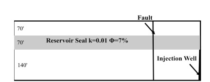
Summary report of probability density functions (development method and outcomes) for an engineered storage site. Given the presence of a major fault located 500 meters from the planned injection site, we will develop probability density functions (PDFs) for risk of (a) leakage through this fault, and (b) induced slip on this fault, following CO₂ injection. We will deliver these PDFs and a detailed description of the process and algorithms used to develop these PDFs.
Generalized Risk Registry (tabulation of risks) for sites with USDWs present.
Detailed (specific) risk registry for the Gordon Creek field site.

Task 4: Hydrodynamic Analysis of Tracer, Microbiologic, Chemistry and Physical Field Data and Use of These Data to Calibrate Quantitative Risk Assessment

Summary report of methods and associated validation approach for tracer, microbiologic, chemical and physical field data used for calibration of quantitative risk assessment.
Brief summary report of approach for application of tracer, microbiologic, chemical and physical field data in reservoir models.
Brief summary report of approach for application of tracer, microbiologic, chemical and physical field in developing risk estimates (in the form of PDFs).

Task 5: Calibration and Refinement of Simulation Models Using Tracer/ Microbiology/Chemistry/Physical Field Data

Summary report of efficacy of gathered data for refining risk estimates in the form of PDFs.

Task 6: Integration and Delivery of Comprehensive Aquifer Risk Assessment Framework (ARAF)

The outcome of Task 6 will be the primary outcome of the entire project: the final ARAF will take the form of a documented protocol for USDW risk assessment published in a summary report. We also will develop a set of companion web-pages to provide practical access to the ARAF. At the end of the project, we will deliver this report and these web-pages to EPA, but we plan to continue updating the framework over the long term.

Task 7: Project Management

Annual reports of progress, followed by the final summary project report.

Task 8: Education and Outreach

A website targeting K-12 students for education regarding geologic CCS, USDWs, potential risks to USDWs, and plans to mitigate those risks.
Presentations at annual project review meetings.
Presentations at national and regional conferences to describe the outcomes of this research to colleagues and other stakeholders.

References:

Allis, R., T. C. Chidsey, W. Gwynn, C. Morgan, S. White, M. Adams, and J. Moore (2001), Natural CO₂ reservoirs on the Colorado plateau and southern Rocky Mountains: candidates for CO2 sequestration.

Altevogt, A. S., and M. A. Celia (2004), Numerical modeling of carbon dioxide in unsaturated soils due to deep subsurface leakage, 40.

Annunziatellis, A., S. E. Beaubien, S. Bigi, G. Ciotoli, M. Coltella, and S. Lombardi (2008), Gas migration along fault systems and through the vadose zone in the Latera caldera (central Italy): Implications for CO₂ geological storage, International Journal of Greenhouse Gas Control, 2, 353-372.

Assayag, N., M. Bickle, N. Kampman, and J. Becker (2009), Carbon isotope constraints on CO₂ degassing in cold-water geyser, Green river, Utah, Energy Procedia, 1, 2361- 2366.

Azzalini, A., and A. W. Bowman (1990), A look at some data on the Old Faithful Geyser, Applied Statistics, 39(3), 357-365.

Bachu, S., and D. B. Bennion (2009), Experimental assessment of brine and/or CO₂ leakage through well cements at reservoir conditions, International journal of Greenhouse Gas Control, 3, 494-501.

Barlet-Gouedard, V., G. Rimmele, O. Porcherie, and J. Desroches (2009), A solution against well cement degradation under CO₂ geological storage environment, International journal of Greenhouse Gas Control, 3, 206-216.

Carroll, J. J., J. D. Slupsky, and A. E. Mather (1991), The solubility of carbon dioxide in water at low pressure, Journal of Physical and Chemical Reference Data, 20(6), 1201- 1209.

Dockrill, B., and Z. K. Shipton (2010), Structural controls on leakage from a natural CO₂ geologic storage site: Central Utah, U.S.A., Journal of Structural Geology.

Duan, Z., and R. Sun (2003), An improved model calculating CO₂ solubility in pure water and aqueous NaClsolutions from 273 to 533 K and from 0 to 2000 bar, Chemical Geology, 193, 257-271.

Ellis, A. J. (1959), The solubility of carbon dioxide in water at high temperature, American Journal of Science, 257, 217-234.

Ellis, A. J., and R. M. Golding (1963), The solubility of carbon dioxide above 100°C in water and in sodium chloride solutions, American Journal of Science, 261, 47-60.

Emberley, S., I. Hutcheon, M. Shevalier, K. Durocher, W. D. Gunter, and E. H. Perkins (2004), Geochemical monitoring of fluid-rock interaction and CO₂ storage at the Weyburn CO₂-injection enhanced oil recovery site, Saskatchewan, Canada, Energy, 29, 1393-1401.

Gasda, S. E., S. Bachu, and M. A. Celia (2004), Spatial characterization of the location of potentially leaky wells penetrating a deep saline aquifer in a mature sedimentary basin, Environmental Geology, 46, 707-720.

Glennon, J. A., and R. M. Pfaff (2005), The operation and geography of carbon dioxide-driven, cold-water "geysers," The GOSA Transactions, IX, 184-192.

Gouveia, F. J., and S. J. Friedmann (2006), Timing and prediction of CO₂ eruptions from crystal geyser, UTRep., Lawrence Livermore National Laboratory.

Han, W. S., G. A. Stillman, M. Lu, C. Lu, B. J. McPherson, and E. Park (2010), Evaluation of potential nonisothermal processes and heat transport during CO2 sequestration, Journal of Geophysical Research, 115(B07209).

Heath, J. E., T. E. Lachmar, J. P. Evans, P. T. Kolesar, and A. P. Williams (2009), Hydrogeochemical characterization of leaking, carbondioxide-charged fault zones in east-central Utah, with implications for geologic carbon storage, in Carbon Sequestration and its Role in the Global Carbon Cycle, edited by B. J. McPherson and E. T. Sundquist, pp. 147-158, American Geophysical Union, Washington, D.C.

Ingebritsen, S. E., and S. A. Rojstaczer (1993), Controls on geyser periodicity, Science, 262, 889-892.

Ingebritsen, S. E., and S. A. Rojstaczer (1996), Geyser periodicity and the response of geysers to small strains in the Earth, Journal of Geophysical Research, 101, 21891- 21907.

Katz, D. L., and R. L. Lee (1990), Natural gas engineering, McGraw-Hill New York. Klusman, R. (2006), Detailed compositional analysis of gas seepage at the National Carbon Storage Test Site, Teapot Dome, Wyoming, USA 21(9), 1498-1521.

Koschel, D., J.-Y. Coxam, L. Rodier, and V. Majer (2006), Enthalpy and solubility data of CO₂ in water and NaCl(aq) at conditions of interest for geological sequestration, Fluid Phase Equilibria, 247, 107-120.

Lu, X., A. Watson, A. V. Gorin, and J. Deans (2005), Measurments in a low temperature CO₂-driven geysering well, viewed in relation to natural geysers, Geothermics, 34, 389- 410.

Mayo, A. L., D. B. Shrum, and T. C. Chidsey (1991), Factors contributing to exsolving carbon dioxide in ground water systems in the Colorado plateau, Utah in Geology of east- central Utah, edited by T. C. Chidsey, Utah Geological Survey, Salt Lake City.

Nordbotten, J. M., M. A. Celia, and S. Bachu (2004), Analytical solutions for leakage rates through abandoned wells, Water Resources Research, 40.

Nordbotten, J. M., M. A. Celia, S. Bachu, and H. K. Dahle (2005), Semianalytical solution for CO₂ leakage through an abandoned well, Environmental Science and Technology, 39, 602-611.

Oldenburg, C. M. (2007), Joule-Thomson cooling due to CO₂ injection into natural gas reservoirs Energy Conversion and Management, 48, 1808-1815.

Oldenburg, C. M., and J. L. Lewicki (2006), On leakage and seepage of CO₂ from geologic storage sites into surface water, 50, 691-705.

Pruess, K. (2008), On CO₂ fluid flow and heat transfer behavior in the subsurface, following leakage from a geologic storage reservoir, Environmental Geology, 54, 1677- 1686.

Rinehart, J. S. (1972), Fluctuations in geyser activity caused by variations in earth tidal forces, barometric pressure, and tectonic stresses, Journal of Geophysical Research, 77, 342-350.

Rinehart, J. S. (1980), Geysers and Geothermal Energy, Springer-Verlag, New York. Rojstaczer, S. A., D. L. Galloway, S. E. Ingebritsen, and D. M. Rubin (2003), Variability in geyser eruptive timing and its causes: Yellowstone National Park, Geophysical Research Letters, 30(18).

Shipton, Z. K., J. P. Evans, D. Kirschner, P. T. Kolesar, A. P. Williams, and J. Heath (2004), Analysis of CO₂ leakage through 'low-permeability' faults from natural reservoirs in the Colorado Plateau, east-central Utah, in Geological Storage of Carbon Dioxide, edited by S. J. Baines and R. H. Worden, pp. 43-58, Geological Society, London.

Shipton, Z. K., J. P. Evans, B. Dockrill, J. Heath, A. Williams, D. Kirchner, and P. T. Kolesar (2005), Natural leaking CO₂-charged system as analogs for failed geologic storage reservoirs, in Carbon Dioxide Capture for Storage in Deep Geologic Formations, edited by D. C. Thomas and S. M. Benson, pp. 699-712, Elsevier, New York.

Waltham, T. (2001), Crystal geyser - Utah's cold one, Geology Today, 17(1), 22-24. Watson, T. L., and S. Bachu (2007), Evaluation of the potential for gas and CO₂ leakages along wellbores, SPE.

White, D. E. (1967), Some principles of geyser activity, mainly from Steamboat springs, Nevada, American Journal of Science, 265, 641-684.

Task 3: Identification of Risk Elements and Development of PDFs

Freethey, G. W.; Cordy, G. E. U.S. Geologic Survey 1991, 1411, 118119.

Pasala, 2010, CO₂ Displacement Mechanisms, Phase Behavior Effects and Carbon Dioxide Sequestration Studies, Ph.D. Dissertation, University of Utah, December 2010.

Task 4: Hydrodynamic Analysis of Tracer, Microbiologic, Chemistry and Physical Field Data and Use of These Data to Calibrate Quantitative Risk Assessment

Hendry, J. M., Kotzer, T. G., and Solomon, D. K., 2005, Sources of radiogenic helium in a clay till aquitard and its use to evaluate the timing of geologic events, Geochimica et Cosmochimica Acta, Vol. 69, No. 2, pp. 475-483.

Osenbrück, J. Lippmann, and C. Sonntag, Dating very old pore waters in impermeable rocks by noble gas isotopes, Geochim. Cosmochim. Acta 62 (1998) 30413045.

Sheldon, A, L. and Solomon, D. K., 2003, Radiogenic helium in shallow groundwater within a clay till, southwestern Ontario, Water Resources Research, Vol. 39, No. 12, 1331, doi:10.1029/2002WR001797.

Journal Articles:

No journal articles submitted with this report: View all 3 publications for this project

Progress and Final Reports:

Original Abstract

The perspectives, information and conclusions conveyed in research project abstracts, progress reports, final reports, journal abstracts and journal publications convey the viewpoints of the principal investigator and may not represent the views and policies of ORD and EPA. Conclusions drawn by the principal investigators have not been reviewed by the Agency.

Grantee Research Project Results

2010 Progress Report: Integrated Design, Modeling, and Monitoring of Geologic Sequestration of Anthropogenic Carbon Dioxide to Safeguard Sources of Drinking Water

Objective:

Progress Summary:

Future Activities:

References:

Journal Articles:

Progress and Final Reports:

Project Research Results

Site Navigation

Related Information