
Grantee Research Project Results
2021 Progress Report: Southeast Wisconsin Interdisciplinary Study of Childrens Health, Ecological Exposures and Social Environment
EPA Grant Number: R839278Title: Southeast Wisconsin Interdisciplinary Study of Childrens Health, Ecological Exposures and Social Environment
Investigators: Magzamen, Sheryl , Carter, Ellison , Jathar, Shantanu , Wilson, Ander , Dilworth-Bart, Janean E
Institution: Colorado State University , University of Wisconsin - Madison
EPA Project Officer: Hahn, Intaek
Project Period: January 1, 2018 through December 31, 2020 (Extended to December 31, 2022)
Project Period Covered by this Report: January 1, 2021 through December 31,2021
Project Amount: $600,000
RFA: Using a Total Environment Framework (Built, Natural, Social Environments) to Assess Life-long Health Effects of Chemical Exposures (2017) RFA Text | Recipients Lists
Research Category: Human Health
Objective:
Objective 1: Develop community- and individual-level profiles for social, physical, and chemical environments and determine the relative associations of these exposure profiles with respiratory, neurodevelopmental, and injury-related outcomes in preschool children in Southeast Wisconsin.
Objective 2: Evaluate the role of community-level social and physical environmental profiles on modification of the effect of chemical exposures on children’s respiratory and neurodevelopmental-related outcomes.
Objective 3: Evaluate the role of residential mobility on respiratory, neurodevelopmental, and physical health in preschool children in Southeast Wisconsin.
Progress Summary:
Outputs of Year 4 are described below. This year’s outputs included moving toward our analytic questions to understand the combination of physical, chemical and social factors on health.
1. Combined air pollution and lead exposure analysis
Our first analysis, led by Research Scientist Dr. Jack Kodros, a new member of our SWISCHEESE team, seeks to understand if there are locations in our study area that are subject to multiple environmental exposures that have deleterious effects on children, namely, blood lead levels and criteria air pollutants. Blood lead levels (bll) for Milwaukee and Racine Counties were retrieved from the Wisconsin Children’s Lead Poisoning Prevention Program; annual mean criteria pollution levels were informed by the InMAP model (Tessum et al. 2017).Understanding the census-tract bll was our first task:
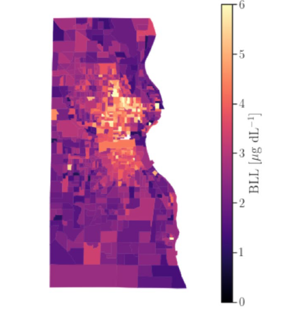
Figure 1. Average blood lead levels for census lock groups in Milwaukee county
Census tracts with higher than average bll tended to be found in the City of Milwaukee region of the study area. The relative standard deviation of BLL in census block groups (CBG) is high (50-100%). This indicates a fair amount of variability in BLL within CBGs, which may suggest a problem with aggregating the BLL dataset from household to CBG levels.
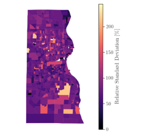
Figure 2. The relative standard deviation in BLL across each census block group
Next, we plotted annual average values of criteria pollutants for the study area (please note that lead was not included as part of the NAAQS exposure due to historically low levels of airborne lead at the current time).
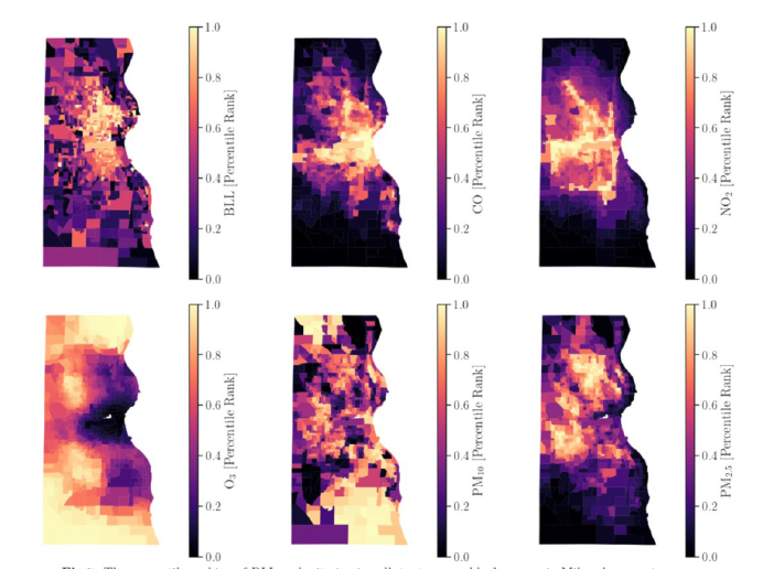
Figure 3. The percentile ranking of BLL and criteria air pollutants across block groups in Milwaukee county
Next, we explored CBGs where BLL and one of the criteria air pollutants are either both above their respective median concentrations or both below their respective median concentrations. He repeated this for IQR instead of median. Next, he colored the CBGs by population density (percentile rankings), non-Hispanic Black population proportion, and non-Hispanic White population proportion.
CBGs where both BLL and one of the air pollutants are above their median values are largely located where there is a high proportion of the non-Hispanic Black population.
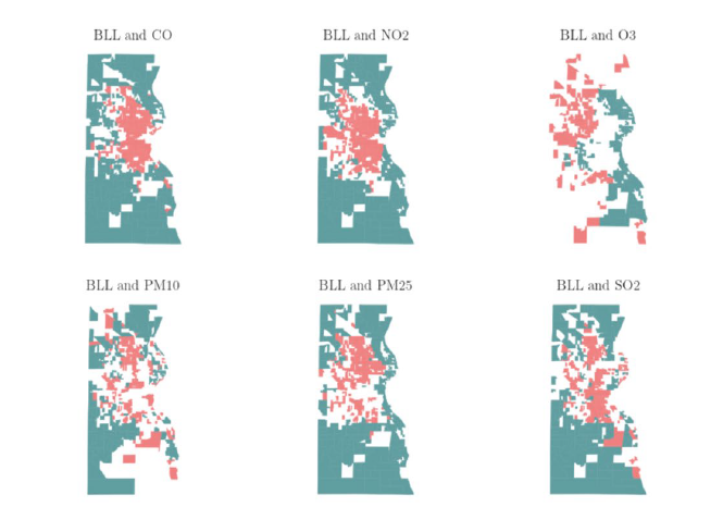
Figure 4. The census block groups where blood lead levels and air pollutant are both above or below their respective median concentrations.
We then corrected for population density:
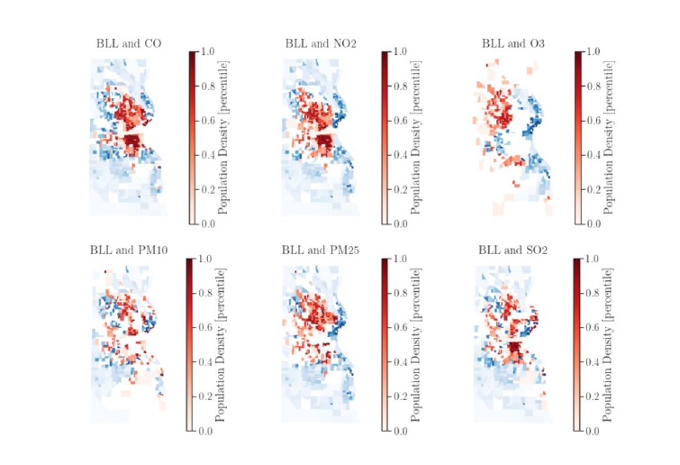
Figure 5. Percentile ranking of population density in CBGs where blood lead levels and an air pollutant are both above/below median concentrations.
Then added population by race, specifically, investigating the proportion of census tract residents who are non-Hispanic Black:
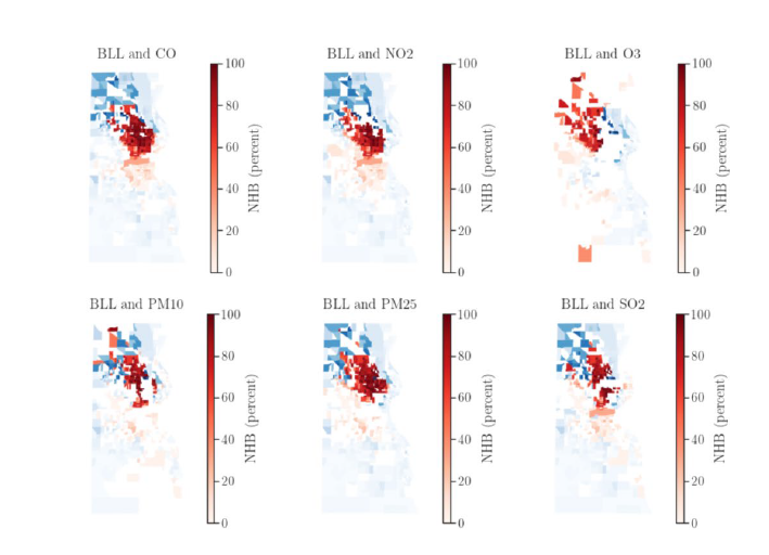
Figure 6. Non-Hispanic Black population fraction in density in CBGs where blood lead levels and an air pollutant are both above/below median concentrations.
In addition to non-Hispanic White populations in the study area. Patterns are quite distinct compared to the non-Hispanic Black populations:
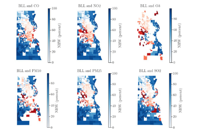
Figure 7. Non-Hispanic white population fraction in CBGs where blood lead levels and an air pollutant are both above/below median concentrations.
A correlation heat maps of bll and air pollutants is provided below:
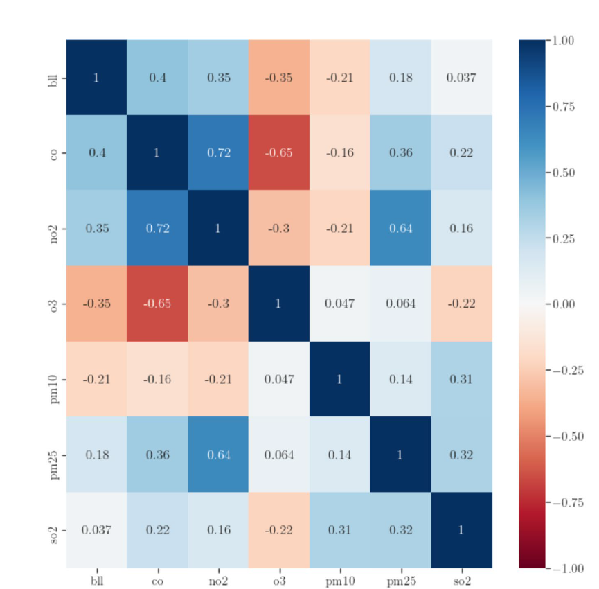
Figure 8. Correlation heatmap of BLL and air pollutants
From ordinal least squares models, we calculated the following:
• A 10% increase in CO is associated with a 19.32% (16.17 - 22.55) increase in BLL
• A 10% increase in NO2 is associated with a 7.20% (5.98 - 8.44) increase in BLL
• A 10% increase in O3 is associated with a -69.51% (-75.49 - -62.07) increase in BLL
• A 10% increase in PM10 is associated with a -8.67% (-11.47 - -5.78) increase in BLL
• A 10% increase in PM25 is associated with a 14.92% (9.91 - 20.16) increase in BLL
• A 10% increase in SO2 is associated with a 2.51% (0.58 - 4.47) increase in BLL
Next, we calculated spatial clustering by pollutants across the study area:
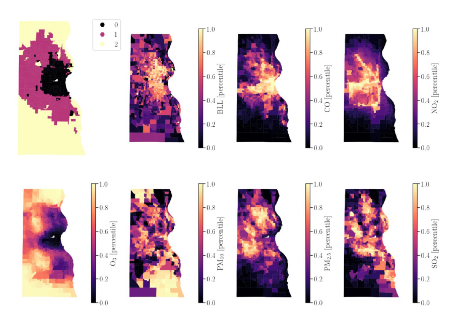
Figure 9. Spatial distribution of clusters along with percentile ranking of BLL and air pollutants
In summary, our findings from the multidomain pollutant analysis indicate:
• Interquartile range of blood lead levels (BLL) in Milwaukee County ranged from 1-4 (μg/dL)
• Though we can perform geocoding to the rooftop level in our study area, household resolution data is very noisy. Aggregating the census block group resolution gives more insight.
• There are weak correlations with BLL and ambient air pollutants (R of 0.4 for CO, -0.35 for O3, 0.2 for PM2.5)
However, there are statistically significant associations of BLL with air pollutants estimate in a linear model
• A 10% increase in in PM2.5 is associated with a 15% (10 - 20) increase in BLL
• A 10% increase in O3 is associated with a 70% (62 - 75) decrease in BLL
• This pattern can be seen in the box-and-whisker plots: the lowest quartile for concentrations of CO, NO2, and PM2.5 are associated with the lowest BLL levels. The opposite is true for O3.
• The K-means clustering algorithm suggests a spatially homogeneous region in the center of Milwaukee County that has the highest BLL levels, CO, NO2 and the lowest O3 and PM1010. PM2.52.5 is also elevated in this region.
• BLL appears to be most strongly associated with air pollutants associated with urban emissions (i.e., CO and NO2).
Dr. Kodros is leading the manuscript development based on the project. We expect to have a manuscript for submission by the end of the calendar year.
1. Lead exposure from multiple built environment features.
SWISCHEESE doctoral student Dr. Tobi Oke (who successfully defended his dissertation in December 2020), based one of his dissertation papers on the SWISCHEESE lead data. In this study, we predicted and improved the interpretability of the contribution of multiple sources and drivers of BLLs using extreme gradient boosting (XGBoost) and Shapley Additive Explanation (SHAP) values to answer the following research questions: (i) what are the relative contributions of each potential source of exposure (i.e., housing characteristics, lead water service lines, and soil lead concentration) to blood lead levels among the children between the ages 1-5 living in Milwaukee; (ii) To what extent do environmental exposure profiles interact synergistically to produce comparatively higher BLL outcomes for children in multiple exposures; and (iii) To what extent this analytical approach can improve lead exposure identification and inform resource allocation to mitigate dominant routes of exposure. XGBoost is one of the intelligent machine learning models seen in various classification or regression studies with high accuracy in prediction models, such as the risk prediction model for type 2 diabetes and breast cancer survival rates.
Blood lead levels.
We obtained the individual level blood lead dataset collected under the Healthy Homes and Lead Poisoning Surveillance system (HHLPSS) from the Wisconsin Department of Health Services, Division of Public Health Services. All the children tested were five years and younger residing in Milwaukee County from 2015 to 2019. The data, which was subject to ethics approval from the Wisconsin Division of Public Health data governance board, record the child's test ID., test date, test type, child's age at the testing date, gender, race, and primary addresses. The BLLs were measured using either venous or capillary testing methods. Some of the BLL values were reported with unknown sampling methods. Therefore, to avoid duplicating samples, if a child had multiple BLL tests, the highest BLL obtained from the venous test was retained since the venous test has been reported to give the most reliable blood lead level result than the capillary method. In addition, if no venous test was performed, the highest BLL obtained from the capillary blood draw was retained. Lastly, if the only test result provided has an unspecified testing method, the test result was used in the analysis—the test results from the unspecified testing method comprised < 2% of all the available test data (Figure 1). After preprocessing the data, 95,659 children were tested for BLL in Milwaukee County, where 71,162 resided within Milwaukee.
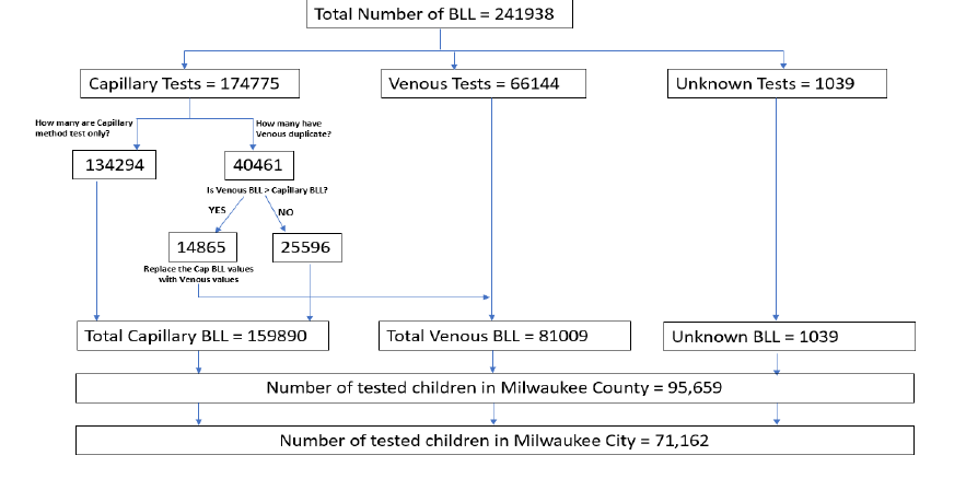
Figure 10. Flow chart showing the data mining process for the Healthy Homes and Lead Poisoning Surveillance blood lead level dataset.
To examine built environment feature's contributions and instances to predicting BLLs, figure 3 displays the magnitude and directions of each instance of a feature SHAP value (i.e., the local interpretability). Each point in the figure corresponds to an instance of a child. Thus, the SHAP value on the x-axis shows whether the effect of that child's feature value contributed to a higher or lower BLL prediction for the child. The red color indicates that the child's feature value is high, while blue indicates lower feature values. For instance, the property value, which was also ranked to have a high overall impact in a model, indicated that children living in houses with low property values have a high and positive impact in predicting the high risks of childhood blood lead poisoning.
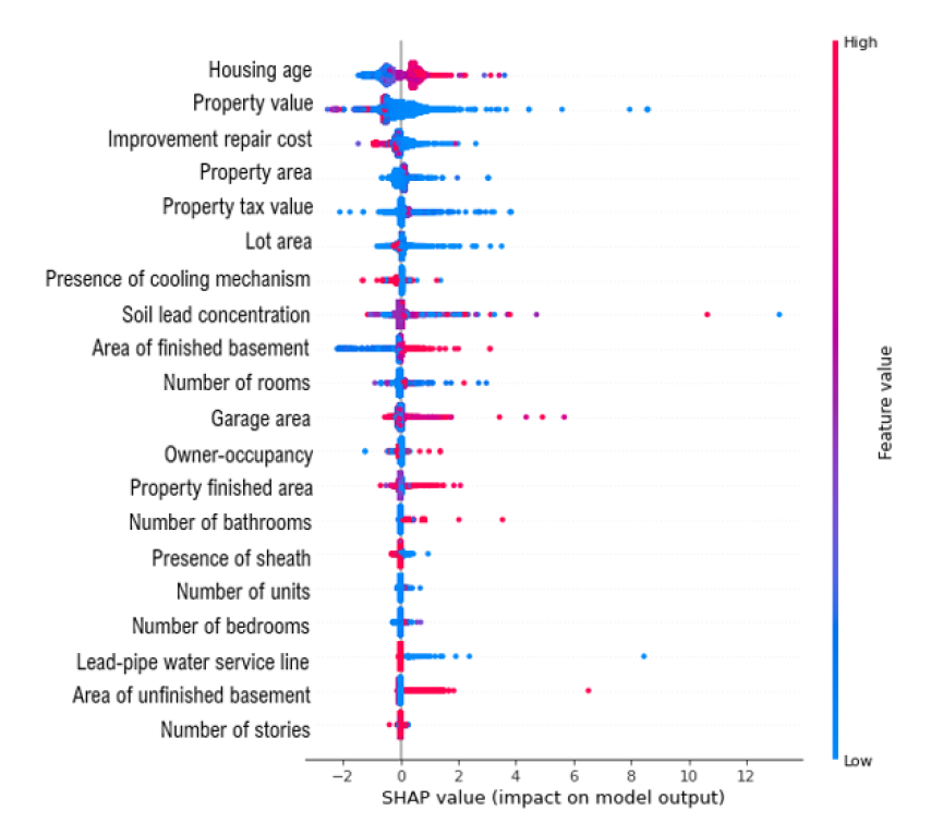
Figure 11. Summary plots for SHAP values. For each feature, one point corresponds to a single child. Thus, a point's position along the x-axis (i.e., the actual SHAP value) represents that feature's impact on the model's output for that specific child. Multiple dots at the same x position pile up to show density.
Our second study, led by Dr. Oke, investigated the contribution of multiple sources and drivers of BLLs using the XGBoost and SHAP values in Milwaukee. We combined the childhood blood lead levels with residential housing characteristics, soil lead concentrations, and lead-pipe and copper-pipe water service lines in Milwaukee. Our first research question focuses on the relative contributions of each source of exposure to blood lead levels among the children between the ages 1-5 living in Milwaukee City. Among the variables considered, housing age (especially those above 90 years old) is the most crucial variable that impacted the prediction of childhood blood lead levels in the city, more than other exposure sources: soil lead concentration and lead-pipe water service lines. These older homes have the potential possibility of having lead-based paints in one or more layers on painted surfaces even though the top paint is lead-free. The result further aligns with a prior study that reported significantly higher rates of pediatric lead poisoning in older housing stocks built before 1950 (72 years ago) in Milwaukee County. In addition, our model output clearly showed that other housing characteristics such as lower property values, improvement values, and tax values are important risk factors or indicators associated with children with lead poisoning. The residents in these kinds of homes have been reported to be low-income and minorities that might not have the financial strength to remodel or mitigate the lead hazards.
Our second research question focuses on how environmental exposure profiles interact synergistically to produce comparatively higher BLL outcomes for children with multiple exposures. For example, the interaction of building age and lead-pipe water service lines influenced the prediction of positive BLLs. Lead abatement treatments and lead-pipe water service lines are expensive for a low-income household to implement and replace. Thus, the interaction of these two multiple exposures could be another significant driver of high pediatric lead poisoning in Milwaukee. In addition, children residing in older homes with replaced lead service lines (blue) have lower SHAP values, indicating that the interaction of older homes and copper service lines could reduce the risk of blood lead. Since the city is replacing the lead-pipe water service lines with copper-pipe, the model output confirms that this approach could effectively reduce pediatric lead poisoning for some exposed kids in Wisconsin, as shown in Figure 4b. Concerning the interaction effect of housing age and soil lead concentration, the SHAP interaction index did not show any clear specific pattern on how the exposure to both sources could be impacting the prediction of childhood blood lead levels. Although some garden soil Pb concentrations are elevated in the study area, these levels might not accurately reflect the indoor Pb-dust concentration that the children are exposed to in their homes.
2. Neighborhood redlining and lead exposure in Milwaukee.
This study, led by SWISCHEESE former postdoctoral scholar Dr. Jeremy Auerbach (now faculty at Queen’s University Belfast) sought to understand how children’s blood lead levels are associated with historical disinvestment in neighborhoods as designated by redlined areas in the study.
Redlining describes discriminatory lending practices of the Home Owner's Loan Corporation (HOLC) during the New Deal era of the 1930s that effectively excluded Black Americans from obtaining government-backed home loans. HOLC created neighborhood security maps of urban areas that described the risk of investment in those areas for over 200 of the largest US cities at the time. Areas with significant Black populations and/or known environmental pollution sources were considered “hazardous” by HOLC standards and did not qualify for federally-backed loans, homeowners' insurance, and home repair or improvement loans. This racist practice created and perpetuated urban racial segregation, restricting the wealth-building of residents and exposing them to hazardous pollutants. The ban of racial discrimination in housing the Fair Housing Act of 1968 could not undo this structural violence perpetrated to these communities and the residents are still impacted by this slow violence today. Furthermore, racist housing strategies have adapted and new ones have emerged, including real estate agent discrimination, the devaluation of Black homes compared to white owned housing, and discriminatory home refinancing practices.
Present-day, these historically redlined neighborhoods are more likely to be communities of color and have higher poverty. Redlined neighborhoods that were classified as “hazardous” have been and are still associated with a lack of protective and healthy built and natural environment features, such as a lack of greenspace, tree canopy, and sidewalks. HOLC D-graded neighborhoods are more likely to be near industrial sources and railroads, and the average number of sources and railroads increases from A to D. The residents of C- and D-grade communities are also exposed to more urban-heat, fire-arm violence, and air pollution. Asthma, cancer, adverse birth outcomes, and overall health is found to be worse in these neighborhoods.
To date, limited research has investigated the links between the practice of redlining and the exposure to lead in one’s home and neighborhood, despite its importance as an environmental risk factor. This analysis explores associations between historical redlining, blood lead levels, and race/ethnicity for children in Wisconsin (US).
We used georeferenced 1930s era HOLC maps developed by the University of Richmond’s Mapping Inequality project to identify HOLC codes in Milwaukee, WI. Mapped neighborhoods were categorized by HOLC into one of four grades: A, best; B, still desirable; C, definitely declining; or D, hazardous for mortgage appraisal. As HOLC neighborhoods vary in number, geographic size, household size, and size of population, a geographic and population weighted analysis was needed. We joined the HOLC grades to individual US Census blocks groups; census block groups provided the smallest spatial resolution of complete Census data1 (geospatial procedures are described in the Supplemental Material). The Census block group data included the number of housing units, the total number of residents, the total number of children (under 18), and the number of children (under 18) by race (White alone, Black alone, Asian alone, and Hispanic or Latino).
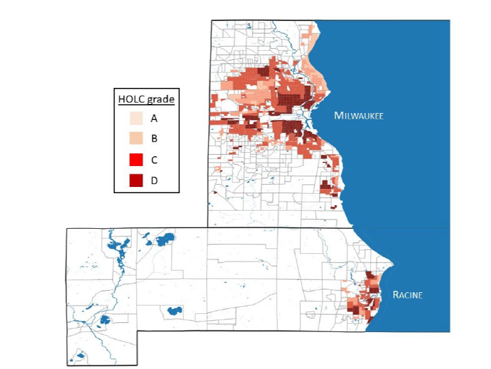
Figure 12. Locations of the HOLC graded neighborhoods in the Milwaukee and Racine counties and cities (WI).
Below are findings from the analysis thus far:
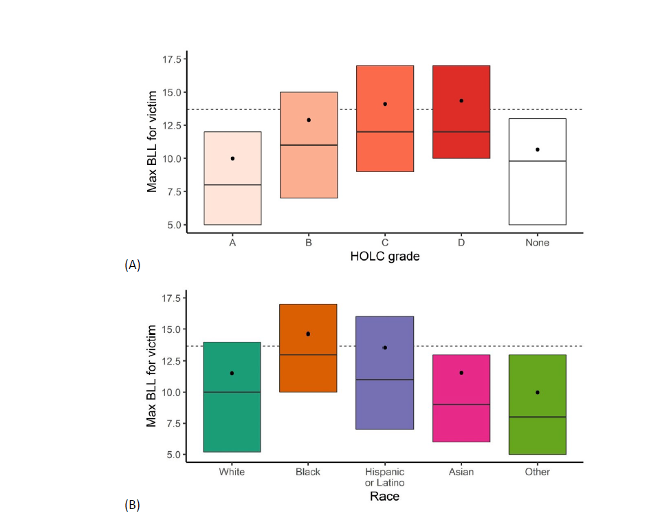
Figure 13. Mean maximum BLLs for the victims stratified by (A) HOLC graded neighborhoods and (B) race and ethnicity. Box plots represent the 25th and 75th percentiles. Medians are indicated with horizontal lines and means by the dot marker; the overall mean maximum is indicated by the dashed horizontal line.
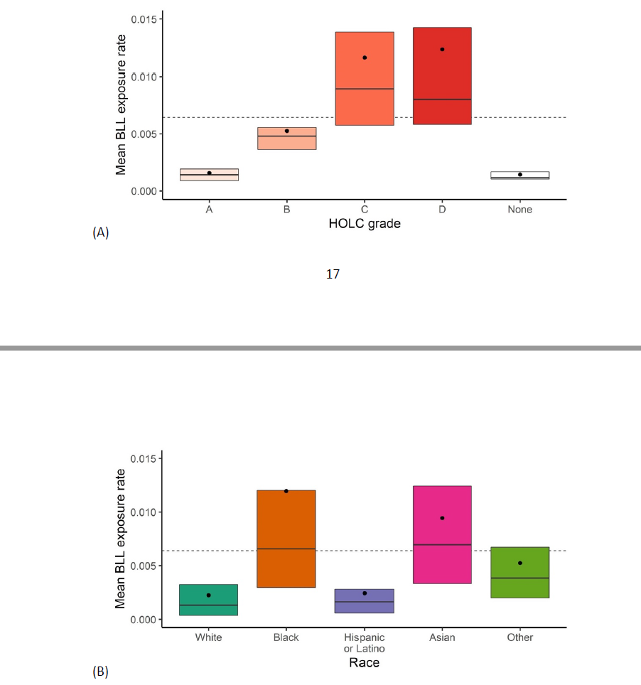
Figure 14. Annual population weighted BLL rates for the victims stratified by (A) HOLC graded neighborhoods and (B) race and ethnicity. Box plots represent the 25th and 75th percentiles. Medians are indicated with horizontal lines and means by the dot marker; the overall mean is indicated by the dashed horizontal line. BLL data was split by year and race.
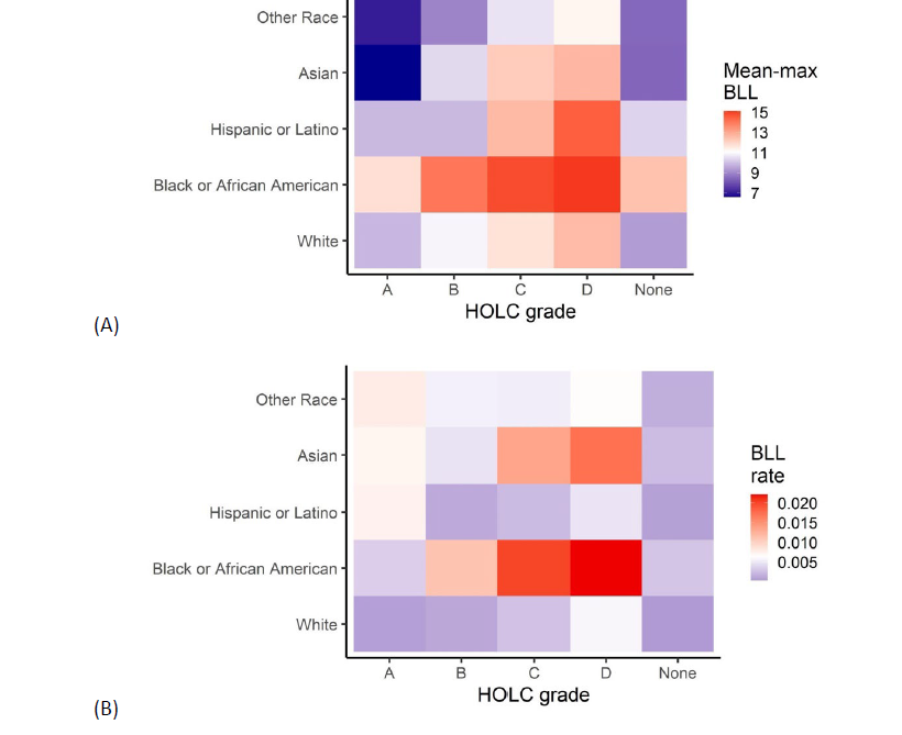
Figure 15. Heatmaps of the BLLs stratified by HOLC grade and race and ethnicity HOLC graded neighborhoods for (A) the mean maximum BLLs and (B) the mean annual population weighted BLL rates. The absence of color identifies the overall mean (mean maximum BLL = 13.7 and mean BLL rate = 0.0065), while a greater intensity of the color blue signifies a lower value from the overall mean and a greater intensity of red for values larger than the overall mean.
. Heatmaps of the BLLs stratified by HOLC grade and race and ethnicity HOLC graded neighborhoods for (A) the mean maximum BLLs and (B) the mean annual population weighted BLL rates. The absence of color identifies the overall mean (mean maximum BLL = 13.7 and mean BLL rate = 0.0065), while a greater intensity of the color blue signifies a lower value from the overall mean and a greater intensity of red for values larger than the overall mean.
Our findings thus far are consistent with a growing body of research linking redlining to racial disparities and adverse environmental health exposures. The increased prevalence of lead exposure in “hazardous” graded neighborhoods is consistent with the lack of abatement brought upon by the lack of investment in these communities. These lead disparities, the structural racism that fostered and maintained them, and the failing policy responses are not unique to the region in this case study.
3. Additional research products.
In addition to these three ongoing projects, we have three additional projects that will be completed with the support of the SWISCHEESE funding. First, working with the Wisconsin Lead Poisoning Prevention Program we have data to conduct an intergenerational analysis to determine if two cohorts of children, those born in 1993 – 1996 who were lead tested are potentially parents or guardians to children born in the study area who have been lead tested. Our goal is to determine if the legacy of lead exposure persists through multiple generations. Second, Dr. Janean Dilworth-Bart is leading an analysis of the role of childhood lead exposure and adult involvement with the court system in Wisconsin. We hypothesize that children who had childhood blood lead levels in the range of concern are disproportionately represented among adults who commit felony and misdemeanor crimes. Lastly, Drs. Magzamen and Carter are leading a paper to understand the lack of progress on healthy homes interventions and policy, using lead as one of the case studies.
Future Activities:
1. Complete DUA with Wisconsin Department of Health Services for use of STELLAR Lead data, WIC data and Medicaid data. (This process has been slowed substantially by the WDHS COVID response in Wisconsin).
2. Complete Data Use Agreement for the Wisconsin Circuit Court Access data (pending).
3. Travel to Milwaukee, WI to conduct Milwaukee Historical Neighborhood tour with David Reimer, former County executive committee.
4. Redevelop timeline based on delays in completing DUA with WDHS.
5. Resubmit all papers listed under Products section (n=6).
6. Develop improved methodological approaches for missing counterfactual population for lead and crime study.
References:
Tessum CW, Hill JD, Marshall JD. InMAP: A model for air pollution interventions. PloS one. 2017 Apr 19;12(4):e0176131.
Journal Articles on this Report : 2 Displayed | Download in RIS Format
| Other project views: | All 8 publications | 7 publications in selected types | All 6 journal articles |
|---|
| Type | Citation | ||
|---|---|---|---|
|
|
KOwalski K, Auerbach J, Martinies S, Starling A, Moore B, Dabelea D, Magzamen S. Neighborhood Walkability, Historical Redlining, and Childhood Obesity in Denver, Colorado. JOURNAL OF URBAN HEALTH-BULLETIN OF THE NEW YORK ACADEMY OF MEDICINE 2023;Early Access |
R839278 (2021) |
Exit |
|
|
Martinies S, Hoskovec L, Wilson A, Moore B, Starling A, Allshouse W, Adgate J, Dabelea D, Magzamen S. Using non-parametric Bayes shrinkage to assess relationships between multiple environmental and social stressors and neonatal size and body composition in the Healthy Start cohort. ENVIRONMENTAL HEALTH 2022;21(1):111 |
R839278 (2021) |
Exit |
Supplemental Keywords:
Medicaid, lead, children, injury, respiratory, neurocognitive, coarsened exact matching, machine learning, indoor air quality, residential mobility, WICProgress and Final Reports:
Original AbstractThe perspectives, information and conclusions conveyed in research project abstracts, progress reports, final reports, journal abstracts and journal publications convey the viewpoints of the principal investigator and may not represent the views and policies of ORD and EPA. Conclusions drawn by the principal investigators have not been reviewed by the Agency.