
Grantee Research Project Results
Final Report: Hydrodynamics of Initial Mixing Zones of Wastewater Discharges
EPA Grant Number: R826216Title: Hydrodynamics of Initial Mixing Zones of Wastewater Discharges
Investigators: Roberts, Philip J.W.
Institution: Georgia Institute of Technology
EPA Project Officer: Aja, Hayley
Project Period: October 1, 1997 through September 30, 2000
Project Amount: $277,643
RFA: Exploratory Research - Physics (1997) RFA Text | Recipients Lists
Research Category: Water , Air , Safer Chemicals , Land and Waste Management
Objective:
The objective of this study was to obtain experimental data on the physics of turbulent mixing processes in buoyancy-modified flows typical of industrial and municipal wastewater discharges. The data consist primarily of laser-induced fluorescence (LIF) images that are converted to tracer concentration fields. The data will be used to refine the mathematical models of dilution and mixing zones used by EPA, and to test the hypothesis that the end of the initial hydrodynamic mixing zone is caused by turbulence collapse under the influence of gravity forces. A new scanning system for generating three-dimensional LIF images has been developed and is described in this report. The system is particularly well suited to studies of jet or plume mixing in stationary or flowing environments.
The experimental system has been fully developed and verified. It consists of laser beam scanners, a high-speed video camera, a computer for image acquisition, and a separate computer for system timing and control. The scanning system consists of two orthogonal galvanometer mirrors that are driven by an analog waveform supplied by a data acquisition card in the control computer. This card controls the overall timing of the system by also sending a synchronized digital signal to control the camera image exposure and image acquisition. The camera is capable of up to 260 frames per second. The original imaging computer had two Xeon processors and 2 gigabytes (GB) of memory to which the images were written directly through a PCI-bus frame grabber made by BitFlow. During the past year, we designed and installed the optics to collimate the laser beam and have been integrating the system components. We have completed thorough testing and calibration of the system; the results of preliminary experiments on round buoyant jets were reported in Roberts and Tian (2000a).
Difficulties were encountered initially because the entire 2 GB of computer memory is not available for image storage; we were not able to record experiments of sufficient duration to obtain stable statistical averages of turbulent quantities. To solve this problem, we took advantage of advances in computer technology that have occurred since the project began, and we designed and specified a new computer system based on faster processing chips, PCI bus data rate, and SCSI hard drives. This system is now fully operational and allows us to stream the images to hard discs (four in parallel) in real time. This is a significant advance, as we are no longer limited by the short duration of the memory-based system. This system was described in Roberts and Tian (2000b).
We have developed software to read and process the image files. This includes the capability to calibrate the pixel response as a function of beam sweep rate and amplitude, exposure time, and dye concentration; and to correct the images for laser attenuation to convert them to quantitative spatial tracer concentration fields, extract time series information at any point, and generate three-dimensional views and animations.
We have thoroughly tested the experimental system and verified it by comparisons with several well-studied flows: a round turbulent jet in a stationary environment, and vertical round buoyant jets in stratified and unstratified crossflows. The system reproduces these previous results closely.
The use of LIF is now a well-established technique for the study of mixing in turbulent flows, particularly jets and plumes. The ability to obtain high spatial and temporal resolution images that yield quantitative information on the instantaneous scalar concentration fields has proven very useful to understanding the mechanics of turbulent mixing processes. Many studies have been reported since the earliest ones by Owen (1976) and Dimotakis, et al. (1983). Most of these studies have been planar LIF (PLIF); information is obtained from images in a two-dimensional plane through the flow. Even relatively simple jet and plume flows are inherently three-dimensional, however, and PLIF cannot reveal this three-dimensionality.
To overcome these difficulties, three-dimensional LIF systems have been under development for some time. In these applications, the laser sheet is swept through the flow at high speed; images are captured with a synchronized camera and saved. Through suitable post-processing and calibration, the three-dimensional concentration field can then be obtained. The first application was possibly Kychakoff, et al. (1987), who studied a laminar premixed flame by scanning the plane of illumination through the flow by an oscillating mirror and obtaining images with an intensified array. Turbulent mixing in homogeneous jets has been studied by Winter, et al. (1987) and Prasad and Srinivasa (1990), who mapped the three-dimensional tracer concentration field by sweeping the sheet through the flow by a rotating mirror and capturing images with a framing camera. More recently, Deusch (1998) studied turbulent mixing, velocity, and velocity gradient using a multipatch 3D image correlation approach.
These early systems were limited to short duration experiments in small areas by image storage capacity and camera sensitivity. As the area illuminated increases, the laser intensity decreases, necessitating either higher laser power or increased fluorescent dye concentrations. Increasing dye concentrations, however, causes further problems in that laser attenuation by the dye increases substantially and calibrations become nonlinear. Maximum image storage often is limited by expensive computer memory. These obstacles gradually have been overcome by recent advances in instrumentation, especially opto-electronics, low-light high-speed cameras, high-speed scanning mirrors, image capture and processing, and mass storage devices. The speed of writing to hard disc has increased rapidly while the cost of hard discs has fallen dramatically; it is now possible to write images to disc in real time, providing (almost) unlimited storage capacity. Whereas it may only have been possible a few years ago to use a dedicated high-speed video system at very high cost, it is now possible to develop even better systems for much lower costs.
Another difficulty with the use of LIF in stratified flows is refractive index variations that arise from density variations and cause random fluctuations in laser intensity. This has limited most studies to situations with small density differences in the flow field, and a small region of interest. These refractive index variation limitations can be overcome by the use of refractive index matching in which liquids of different density but equal refractive index are used. We do refractive index matching with ethanol and salt (NaCl) solutions. The main advantage of using ethanol and salt is lower cost, which is important when large volumes are needed. Ethanol, however, results in a substantial decrease in laser power due to attenuation; this can be corrected by using the methods described in Daviero, et al. (1999).
In this report, the development and some applications of the three-dimensional scanning system for imaging of jet and plume flows in a stratified towing tank are described. The source is towed through the stationary water in the tank; the camera is attached to the towing carriage so that it is stationary relative to the source. In the examples given, the discharge is a vertical round buoyant jet in a homogeneous or linearly stratified crossflow. This flow was chosen because it is an important flow with many applications in air and water pollution control, and it has been extensively studied so much data are available for comparison.
Summary/Accomplishments (Outputs/Outcomes):
Experimental System
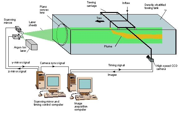
A schematic depiction of the experimental configuration is shown in Figure 1. The glass-walled tow tank is 6.10 meters long by 0.91 meters wide by 0.61 meters deep. The tank is housed in a specially built darkroom to eliminate ambient light. The tow tank has two 3-meter-long glass panels to enable long duration tows with unobstructed views of the flow. A tow carriage powered by a variable speed DC electric motor carriage runs on smooth bearings on precision stainless steel rods the length of the tank. The tank framework is painted with black epoxy paint to resist corrosion and to reduce reflections. The effluent, a mixture of water, salt, and fluorescent dye, is supplied from a reservoir by a rotary pump. The flowrate is measured by a precision rotameter. The tank can be linearly stratified using a two-tank filling system (Daviero, 1998). The strength of the stratification was measured either by traversing the fluid with a conductivity probe or by measuring the densities of samples extracted from various depths with a Troemner-specific gravity balance.
The LIF system uses a continuous wave Argon-Ion laser. The laser is a Lexel 95-4 Argon-Ion laser with nominal maximum power in all-line mode of about 4 W. We use it in single-line mode in the green line (514 nm) with a power of about 2 W. The fluorescent dye is Rhodamine 6G, which has peak absorption at about 530 nm and peak emission at about 560 nm. Characteristics of this dye are given in Ferrier, et al. (1993). Small amounts of the dye are added so that dye concentrations in the diluted jet are low, typically around 10 mg/L. The laser sheet causes the dye to fluoresce, and the emitted light is captured by a CCD camera. The CCD camera is attached to the tow carriage and moves with it so that the discharge appears to be stationary relative to the camera. A long pass orange filter (Schott glass 530) is placed over the camera lens to pass only the fluoresced light and eliminate the laser scattered light.
The LIF system is controlled by two computers-one for overall timing control and one for image capture. The timing control computer contains a National Instruments Multifunction I/O Board to provide the timing control and an analog voltage signal to drive the scanning mirrors. This analog signal is converted at a resolution of 12 bits from a digital file. The scanning mirrors consist of two orthogonal fast galvanometer mirrors made by Cambridge Technology. The first mirror drives the beam in the horizontal (y) direction, the second in the vertical (z) direction. After leaving the scanning mirrors, the beam strikes a large plano-convex lens 350 mm in diameter with a focal length of 940 mm. The distance from the scanning mirrors to this lens is equal to the focal length of the lens; wherever the beam strikes the lens, it is refracted parallel to the axis of the tow tank. In practice, this is not quite possible, as the virtual beam location relative to the lens moves as the mirrors scan. This movement is quite small relative to the focal length of the lens, however, so deviations from parallel are small.
The CCD camera is a Dalsa CA-D6. The resolution (number of active pixels) is 530 by 515. It is a digital camera that provides output in 8-bit resolution-a gray scale with 256 levels. The data format is Low Voltage Differential Signal ([LVDS], also known as EIA-644), which enables high-data transmission rates over long cable lengths. The maximum frame rate of this camera is 260 frames per second, which gives a maximum data rate of about 71 MHz. We usually use it at 100 or 200 frames per second. It achieves this high data rate by using four taps, each capable of 25 MHz. The camera can be externally triggered, which is how it is used here.
Figure 1. Schematic Depiction of Experimental Arrangement
It has a high-gain A/D converter to enable use with low fluorescence light levels. Even with the high gain, the noise level is still quite low. For the experiments reported here, a Fujinon CCTV camera lens of 25 mm focal length and f0.85 aperture was used.
The frame grabber board is a Bitflow RoadRunner. Video Savant software is used to control image capture and saving. Initially, images were written to computer memory in real time and later saved to hard disc. This computer had 2 GB of memory on the motherboard, of which about 1.6 GB was actually available for images storage. Therefore, the system was limited to about 6,500 images, which corresponds to about 30 seconds of data at 200 frames per second, or 60 seconds at 100 frames per second. We have since developed a real-time-to-disc system that allows streaming the images to disc in real time. This allows much longer experimental durations.
The laser and image acquisition are controlled and synchronized as follows. The I/O Board sends a TTL signal to the frame grabber board to initiate frame capture, and the frame grabber board in turn sends an LVDS signal to the camera to begin image acquisition (exposure). Simultaneously, the I/O Board begins sending an analog voltage to move the vertical (z) mirror. The beam makes one sweep down and back while the camera is exposing (i.e., the shutter is "open"). A voltage is then sent to the horizontal (y) mirror to move the beam a small distance horizontally. The cycle then begins again with another TTL signal that downloads the previous frame, clears the camera buffer, and begins the next exposure. This is repeated so that multiple vertical "slices" through the flow are obtained. After a predetermined number of "slices," the beam returns to the starting point and the cycle starts again. For example, 20 slices at 200 frames per second yields an effective sample rate, at which the whole sequence of images through the flow is captured, of 10 Hz.
There are tradeoffs between the height of the area imaged, the camera frame rate, and the dye concentration. As the height is increased, the laser intensity at any point decreases, and as the frame rate increases, the exposure time decreases. Both of these reduce the light level reaching the camera. Increasing dye concentrations can compensate for this, but for quantitative work, it is desirable to keep the dye concentrations below about 50 mg/L if possible. Beyond these levels, the light output as a function of dye concentration becomes nonlinear and attenuation of the laser by the dye increases rapidly (Ferrier, et al., 1993). We maximized the light reaching the camera by using a fast (f0.85) lens and a sharp cutoff filter (Schott Glass 530) that passes most of the fluoresced light while blocking the scattered laser light. For example, a dye concentration of 120 mg/L causes pixel saturation with a laser power of 2 W, a sheet height of 230 mm, and a frame rate of 100 frames per second.
Quantitative scalar concentration data are obtained by calibration. We capture images of a tall cylinder containing known amounts of dye placed in the towing tank, similar to the procedure of Ferrier, et al. (1993). A pixel-by-pixel calibration in which corrections for lens luminance variation (vignetting) and individual pixel response is then done. Finally, the images are corrected for attenuation due to clear water, dye, salt, and ethanol, using the methods of Daviero, et al. (1999). The multiple "slices" through the flowfield are then regenerated, using three-dimensional image processing software, into a three-dimensional image of the flow. The time of scanning through the flow is sufficiently short to "freeze" the larger turbulent scales.
Applications
To illustrate the system, two applications are given of a round buoyant jet into unstratified and stratified crossflows. The experiments are performed as shown in Figure 1, in which a more dense effluent is discharged downwards. The results are reported here as inverted, that is, as a positively buoyant effluent discharging upwards. This is allowable because the relative density difference between the effluent and receiving water is small and is therefore significant only for buoyancy forces and not inertia forces (the Boussinesq assumption).
For both experiments, the nozzle diameter d was 0.42 cm, the current speed u was 4.0 cm/s, and the effluent flowrate Q was 6.31 cm3/s. For the unstratified experiment, the density difference between the effluent and ambient was 14.7 kg/m3, and for the stratified experiment was 16.3 kg/m3. For the stratified experiment, the density profile was approximately linear with a buoyancy frequency, N=-g d ρ---ρο dz = 0.46 s-1, where g is acceleration due to gravity, r0 is a reference density, taken as 1,000 kg/m3, and dr/dz is the vertical density gradient. This yields the following parameters: Jet Reynolds number, Re = 1900, buoyancy flux, B = g(Δρ/ρ)Q=91.0 cm4/s (unstratified), and 101 cm4/s (stratified), and momentum flux, M = υ;Ο = 287 cm4/s2, where μj is the jet velocity. Relevant length scales for the flow (Wright, 1984) are: ιb = B/υ3 = 1.42 cm (unstratified) = 1.58 cm (stratified), and ιm = Mιη/ υ =4.24 cm. For the stratified flow, two further length scales are ιm' = M1/4/Niη = 6.1 cm and ιb' = Bι/4/N3/4 = 5.5 cm. Both the buoyancy and momentum fluxes are therefore important for this particular flow.
For both experiments, the height of the laser sheet was 23 cm, the thickness about 2 mm, the horizontal distance between laser sheets was 0.87 cm, and 20 sheets were imaged per full sequence for a total width imaged of about 16.5 cm. The camera frame rate was 100 frames per second, and 2,800 images were captured for 28 seconds. The source dye concentration was 600 mg/L and 800 mg/L for the unstratified and stratified cases, respectively. The camera saturated near to the nozzle so no quantitative data were obtained there.
Results
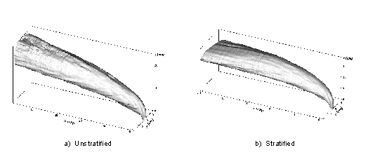
Quantitative measurements of the tracer concentration field have been made for a round jet in an unstratified, stationary environment. These are reported in Roberts and Tian (2000a). Three-dimensional visualizations of the outer surfaces of the jets are shown in Figure 2. Similar time-averaged views are shown in Figure 3. In these figures, the surface threshold level is set just above zero. The unstratified jet shows a familiar shape and trajectory; the stratified jet shows flattening near its terminal rise height.
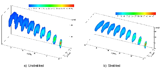
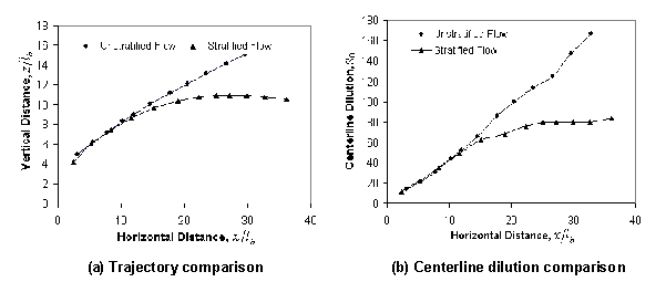
Once three-dimensional data like these are obtained, a great amount of information can be extracted from it. For example, Figure 4 shows vertical profiles of tracer concentration at various distances from the source. Color-coding shows constant contours of tracer levels. The familiar kidney shapes are apparent, with the maximum concentrations appearing to the sides of the vertical plane through the jet centerline. Trajectories also can be obtained. Figures 5 and 6 show centerline trajectories and dilutions for the two cases and comparisons with the asymptotic solutions of Wright (1984). These data will be reported in future papers. This information should be of great value in improving mathematical plume models.
Figure 2. Renderings of instantaneous threshold concentration surface of unstratified and stratified jets.
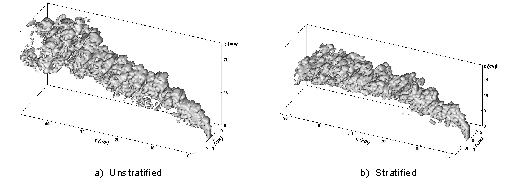
Figure 3. Renderings of time-averaged threshold concentration surfacea of unstratified and stratified jets.
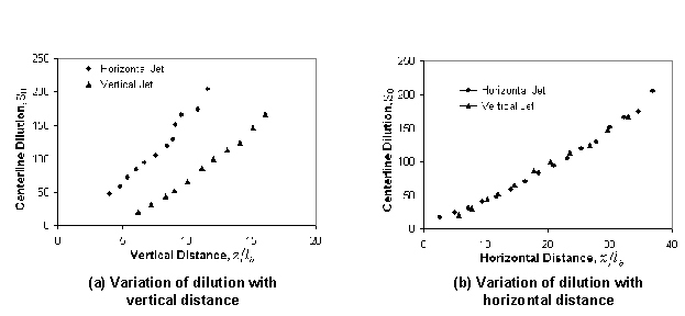
We also have studied a horizontal buoyant jet directed normal to the crossflow (i.e., with a three-dimensional trajectory). Comparisons of the variation of dilution with distance between the horizontal and vertical jet are shown in Figure 7.
Quality Assurance
Quality assurance has been ensured by following the procedures of the original Quality Assurance Statement. The criterion for LIF data acceptance is an agreement within about 20 percent with that obtained by other techniques. The measurements are made in a density-stratified towing tank under conditions typical of wastewater discharges into various hydrological environments. The measurements are of tracer concentrations by LIF. A small amount of fluorescent dye, Rhodamine 6G, is added to the effluent. The laser causes the dye to fluoresce, and the fluoresced light is captured by a sensor and digitized. A long pass optical filter ensures that only the fluoresced light is passed, and not that scattered by particles in the flow field. Typical dye concentrations are of the order of 10 mg/L. The local tracer concentration is computed from the sensor response after corrections. The laser power at the laser head is monitored continuously throughout the experiment by an internal photocell whose analog output is digitized at 12 bits to ensure a steady power output during the experiment.
Figure 4. Vertical concentration profiles through unstratified and stratified jets.
Fluid densities are measured by a Mettler Specific Gravity Balance to an absolute precision of 0.1 σt-units (0.0001 g/cc). The tank is stratified by a two-tank filling system and the stratification is measured by the conductivity probe whose height is measured with a vernier scale to a precision of 0.01 inches. Effluent flowrate is measured by a flowmeter that is calibrated volumetrically to an accuracy of ?3 percent. The tow speed is measured by timing the travel of the towing carriage over a measured distance.
Because this is an in situ method of measurement, no samples from the flow field are obtained. The measurements are made in a nonintrusive manner, with no contact with the flow. No samples are stored for long periods; therefore, there is no custody or handling of samples.
The LIF system is calibrated by obtaining images of a triple-cell filled with three dye solutions of known concentration. A concentrated dye solution is first made by adding dye, whose weight is measured on a precision balance, to water, whose volume is measured in calibrated measuring cylinders. Samples of lower concentrations are then made by sequential dilution in which the concentrated solution is diluted in larger volumes of water. All volume measurements are made by calibrated measuring cylinders. The solutions are stored in dark brown bottles to avoid any reduction in fluorescence by photochemical decay. The water is dechlorinated prior to adding the dye to avoid quenching by chlorine.
To obtain tracer concentration levels from the fluorescence, further data reduction is necessary. This consists of corrections for a number of effects, including: spatial variation in laser sheet intensity; spatial attenuation of the laser sheet; spatial variation in lens response (vignetting); and noise, including random and electronic and background fixed pattern noise (BFPN). The attenuation of the beam as it passes through the tank is exponential. We have measured the attenuation coefficient as a function of ethanol, salt, and dye concentration by measuring the decrease in laser intensity as it passes through the 20-foot-long towing tank. The sheet intensity varies spatially due to the nonlinear sweep velocity of the beam, which causes the integrated amount of light received by the sensor to vary spatially. This spatial variation is obtained by the triple-cell calibration images discussed above.
Figure 5. Comparisons of trajectory and dilution of vertical bouyant jets un unstratified crossflows.
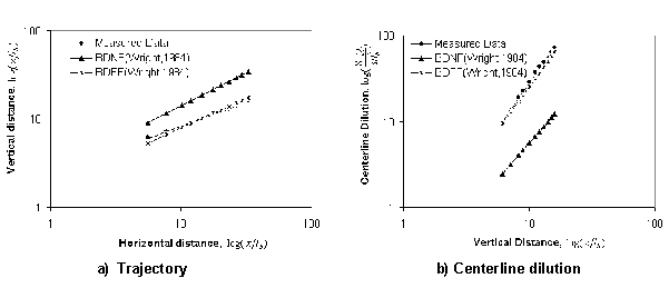
Figure 6. Trajectories and dilutions of vertical bouyant jets in unstratified and stratified crossflows.
The data are cataloged and archived on Travan Tape cartridges, along with the experimental conditions for each experiment.
We have thoroughly tested the experimental system and verified it by comparisons with several well-studied flows: a round turbulent jet in a stationary environment, and vertical round buoyant jets in stratified and unstratified crossflows. The system reproduces these previous results to within about ? 15 percent, and is therefore judged acceptable.
Figure 7. Dilution of horizontal and vertical bouyant jets in unstratified crossflows.
Conclusions:
A scanning laser system has been developed to enable three-dimensional LIF imaging in fairly large-scale turbulent stratified flows. This now can be done at reasonable cost due to recent instrumentation advances, particularly in scanning mirrors, high-speed low-light CCD cameras, and image acquisition and storage.
Example applications to round buoyant jets discharging into unstratified and stratified crossflows are reported. Detailed analyses of these flows will be reported later. We plan to apply the system to a wide variety of jet and plume problems related to the discharge and mixing zones of wastewaters in the environment.
References:
Daviero G. Hydrodynamics of ocean outfall discharges in unstratified and stratified flows. Ph.D. Thesis, School of Civil Engineering, Georgia Institute of Technology, 1998.
Daviero GJ, Roberts PJW, Maile K. Refractive index matching in large-scale stratified experiments. Experiments in Fluids 1999 (submitted for publication).
Deusch S. Imaging of turbulent mixing by laser induced fluorescence and application to velocity and velocity gradient measurements by a multi-patch 3D image correlation approach. Ph.D. Thesis, Georgia Institute of Technology, 1998.
Dimotakis PE, Miake-Lye RC, Papantoniou DA. Structure and dynamics of round turbulent jets. Physics of Fluids 1983;26(11):3185-3192.
Ferrier AE, Funk D, Roberts PJW. Application of optical techniques to the study of plumes in stratified fluids. Dynamics of Atmospheres and Oceans 1993;20:155-183.
Kychakoff G, Paul PH, van Cruyningen I, Hanson RK. Movies and 3-D images of flowfields using planar laser-induced fluorescence. Applied Optics 1987;26(13):2498-2501.
Owen FK. Simultaneous laser measurements of instantaneous velocity and concentration in turbulent mixing flows. AGARD-CP193, Paper No. 27.
Prasad RR, Srinivasa KR. Quantitative three-dimensional imaging and the structure of passive scalar fields in fully turbulent flows. Journal of Fluid Mechanics 1990;216:1-34.
Roberts PJW, Tian X. Three-dimensional imaging of stratified plume flows. Presented at the 5th International Conference on Stratified Flows, Vancouver, British Columbia, July 10-13, 2000(a).
Roberts PJ, Tian X. New experimental techniques for outfall plume flows. Presented at the International Conference MWWD2000 - Marine Wastewater Discharges, Genova, Italy, November 28-December 1, 2000(b).
Winter M, Lam J, Long M. Techniques for high-speed digital imaging of gas concentrations in turbulent flows. Experiments in Fluids 1987;5(3):177-183.
Wright SJ. Buoyant jets in density-stratified crossflow. Journal of Hydraulic Engineering 1984;110(5):643-656.
Journal Articles:
No journal articles submitted with this report: View all 2 publications for this projectSupplemental Keywords:
water, toxics, discharge, mixing zone, mathematical models, dilution., Scientific Discipline, Water, Environmental Chemistry, Wastewater, Hydrology, Physics, municipal wastewater treatment, three dimensional model, dilution, estuaries, industrial wastewater, wastewater discharges, initial mixing zones, mathematical model, high speed imaging, discharge, National Pollutant Discharge Elimination System (NPDES), laser induced fluorescence, hydrodynamicsProgress and Final Reports:
Original AbstractThe perspectives, information and conclusions conveyed in research project abstracts, progress reports, final reports, journal abstracts and journal publications convey the viewpoints of the principal investigator and may not represent the views and policies of ORD and EPA. Conclusions drawn by the principal investigators have not been reviewed by the Agency.